Tutorials
This section provides step-by-step tutorials for using Planet Ruler to determine planetary radius from horizon photographs using the default interactive manual annotation approach.
Tutorial 0: Pre-Configured Earth Radius Measurement
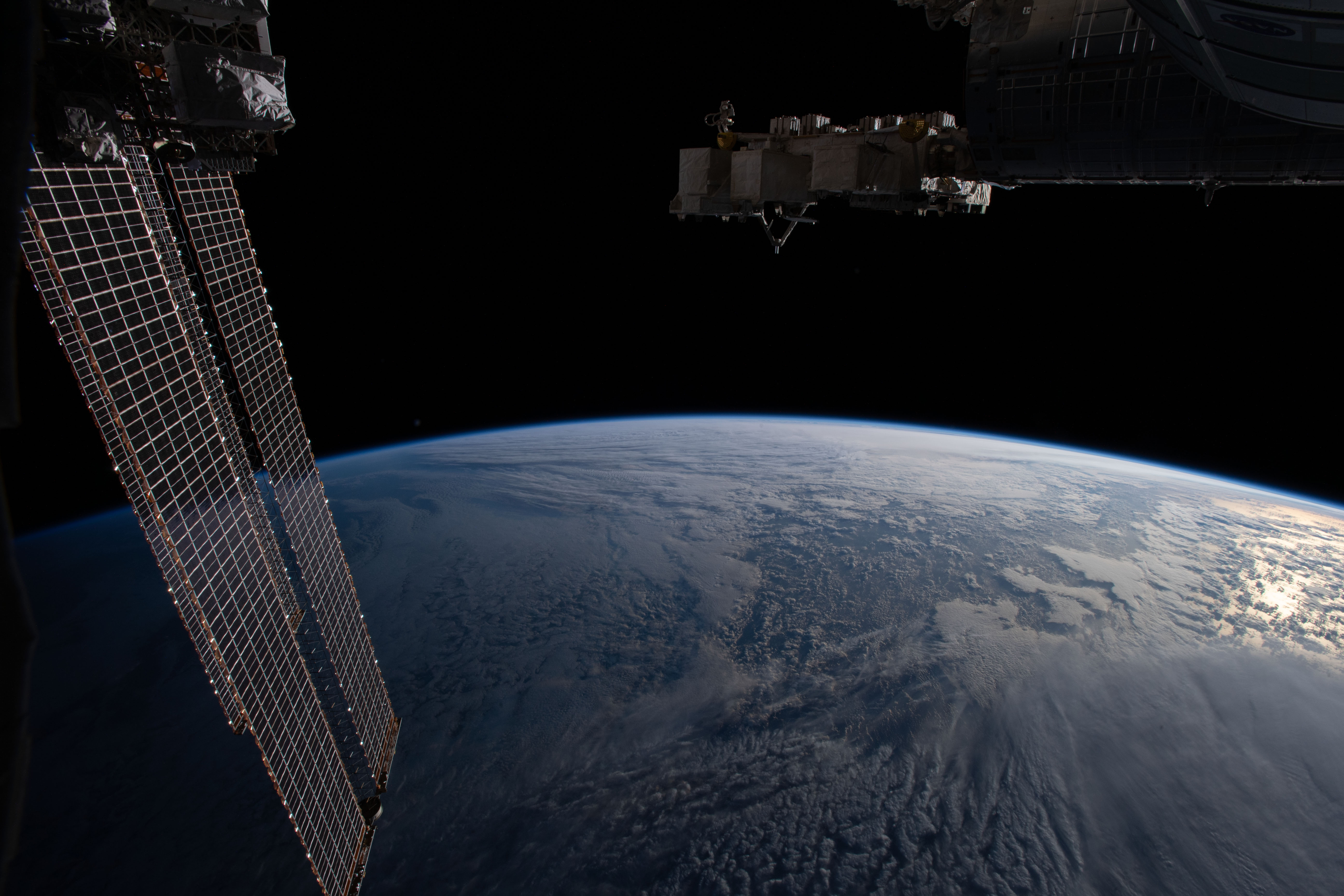
This tutorial shows how to calculate Earth’s radius using a horizon photograph with known altitude and camera parameters via the default interactive manual annotation method.
Prerequisites
Python 3.10+ with Planet Ruler installed (no additional dependencies needed)
A horizon photograph (we’ll use the demo Earth image)
Basic knowledge of the observation altitude
Note
Manual vs Automatic Methods: Planet Ruler’s default manual annotation provides precise, user-controlled horizon detection with no additional dependencies. For automated processing, gradient-field and AI segmentation (requires PyTorch + Segment Anything) detection are also available.
Step 1: Setup and Imports
import planet_ruler.observation as obs
import planet_ruler.geometry as geom
from planet_ruler.uncertainty import calculate_parameter_uncertainty
from planet_ruler.fit import format_parameter_result
import matplotlib.pyplot as plt
Step 2: Load Configuration and Image
Planet Ruler uses YAML configuration files to specify camera parameters and initial estimates:
# Load Earth ISS observation
observation = obs.LimbObservation(
    image_filepath="demo/images/ISS_Earth_horizon.jpg",
    fit_config="config/earth_iss_1.yaml"
)

# Display the loaded image
observation.plot()
The configuration file contains:
Camera specifications: focal length, detector width, field of view
Initial parameter estimates: planet radius, observation altitude
Optimization settings: free parameters, parameter bounds
Step 3: Detect the Horizon (Default: Manual Annotation)
Planet Ruler offers three detection methods, with manual annotation as the default:
# Method 1: Manual annotation (default - precise, no dependencies)
observation.detect_limb(detection_method="manual")  # Opens interactive GUI

# Method 2: Gradient-field (automated - good for clear horizons)
# Here you get to skip detection! This method fits the planet radius to the image
# directly so no need to identify the limb.

# Method 3: AI segmentation (automated - requires PyTorch)
# observation.detect_limb(detection_method="segmentation")
# observation.smooth_limb(
#    method="rolling-median",
#    window_length=15,
#    fill_nan=True
# )

# Plot the detected limb
observation.plot()
Tip
Method Comparison:
Manual: Precise user control, works with any image quality, no dependencies
Gradient-field: Automated, fast, works with clear horizons, no ML dependencies
Segmentation: Most versatile, handles complex images, requires PyTorch + Segment Anything
Step 4: Fit Planetary Parameters
Now we optimize the planetary radius to match the observed horizon curvature:
# Perform the fit
observation.fit_arc(
    minimizer="differential-evolution",
    seed=42  # For reproducible results
)

print("Fit completed successfully!")
print(f"Fitted parameters: {observation.best_parameters}")
Monitoring Progress with Dashboard:
For long optimizations, enable the live progress dashboard via fit_limb
with an explicit stages list:
# Enable dashboard for real-time monitoring
observation.fit_limb(
    stages=[{"method": "arc", "minimizer": "differential-evolution"}],
    dashboard=True  # Shows live progress
)

# Configure dashboard display
observation.fit_limb(
    stages=[{"method": "arc"}],
    dashboard=True,
    dashboard_kwargs={
        'width': 80,         # Wider display
        'max_warnings': 5,   # More warning slots
        'max_hints': 4,      # More hint slots
    }
)
The dashboard shows: - Current parameter estimates - Loss reduction progress - Convergence status - Warnings and optimization hints - Adaptive refresh rate (fast during descent, slow at convergence)
Tip
Faster convergence with staged fitting: chain a quick sagitta estimate into the arc fit to narrow the search space automatically:
observation.fit_limb(
    stages=[
        {"method": "sagitta"},
        {"method": "arc", "minimizer": "differential-evolution"},
    ]
)
Step 5: Calculate Uncertainty
Planet Ruler provides multiple uncertainty estimation methods:
from planet_ruler.uncertainty import calculate_parameter_uncertainty

# Auto-select best method (population for DE, hessian for others)
radius_result = calculate_parameter_uncertainty(
    observation,
    parameter="r",
    scale_factor=1000,  # Convert to kilometers
    method='auto',
    confidence_level=0.68  # 1-sigma
)

print(f"Radius: {radius_result['uncertainty']:.1f} km")
print(f"Method used: {radius_result['method']}")

# Alternative methods:

# 1. Population spread (fast, exact for differential-evolution)
pop_result = calculate_parameter_uncertainty(
    observation, "r",
    scale_factor=1000,
    method='population',
    confidence_level=0.68
)

# 2. Hessian approximation (fast, works with all minimizers)
hess_result = calculate_parameter_uncertainty(
    observation, "r",
    scale_factor=1000,
    method='hessian',
    confidence_level=0.68
)

# 3. Profile likelihood (slow, most accurate)
profile_result = calculate_parameter_uncertainty(
    observation, "r",
    scale_factor=1000,
    method='profile',
    confidence_level=0.68,
    n_points=20
)

# Get confidence intervals at different levels
for cl in [0.68, 0.95, 0.99]:
    result = calculate_parameter_uncertainty(
        observation, "r",
        scale_factor=1000,
        method='auto',
        confidence_level=cl
    )
    print(f"{int(cl*100)}% CI: ± {result['uncertainty']:.1f} km")
Step 6: Validate Results
Compare your results with the known Earth radius:
known_earth_radius = 6371.0  # km
fitted_radius = radius_result["value"]
uncertainty = radius_result["uncertainty"]

error = abs(fitted_radius - known_earth_radius)
error_in_sigma = error / uncertainty

print(f"Known Earth radius: {known_earth_radius} km")
print(f"Fitted radius: {fitted_radius:.1f} ± {uncertainty:.1f} km")
print(f"Absolute error: {error:.1f} km")
print(f"Error in standard deviations: {error_in_sigma:.1f}σ")

if error_in_sigma < 2.0:
    print("✓ Result is within 2σ of known value!")
else:
    print("⚠ Result differs significantly from known value")
Expected Results: For Earth from ISS altitude (~418 km) using manual annotation: * Fitted radius: ~6,371 ± 15 km (high precision from careful point selection) * Error: < 50 km from true radius
Tutorial 1: Auto-Configured Earth Radius Measurement
The fastest way to get started using your own images with Planet Ruler by using automatic camera parameter detection from EXIF data.
Prerequisites
Python 3.10+ with Planet Ruler installed
A horizon photograph with EXIF data (from phone, DSLR, mirrorless camera)
Known or estimated altitude when photo was taken
Step 1: Automatic Camera Detection
Planet Ruler can automatically extract camera parameters from image EXIF data:
from planet_ruler.camera import create_config_from_image

# Automatically generate config from image EXIF
auto_config = create_config_from_image(
    image_path="your_horizon_photo.jpg",
    altitude_m=10_000,  # Your altitude in meters
    planet="earth",
    limits_preset="balanced",  # "tight", "balanced" (default), or "loose"
)

# View detected camera info
print("Auto-detected camera:")
camera_info = auto_config["camera_info"]
print(f"  Model: {camera_info.get('camera_model', 'Unknown')}")
print(f"  Type:  {camera_info.get('camera_type', 'Unknown')}")
# Focal length and sensor width are stored in meters in init_parameter_values
f_mm = auto_config["init_parameter_values"]["f"] * 1000
w_mm = auto_config["init_parameter_values"]["w"] * 1000
print(f"  Focal length: {f_mm:.1f} mm")
print(f"  Sensor width: {w_mm:.1f} mm")
Step 2: Direct Analysis (No Config Files)
Use the auto-generated configuration directly:
import planet_ruler.observation as obs

# Load observation using auto-generated config
observation = obs.LimbObservation(
    image_filepath="your_horizon_photo.jpg",
    fit_config=auto_config  # Use dict instead of file path
)

# Standard workflow
observation.detect_limb(detection_method="manual")
observation.fit_arc()
Step 3: CLI Usage (Even Simpler)
For the simplest workflow, use the command line:
# One command to measure planetary radius
planet-ruler measure --auto-config --altitude 10000 --planet earth your_photo.jpg

# Override auto-detected field-of-view if needed
planet-ruler measure --auto-config --altitude 10000 --planet earth --field-of-view 60 your_photo.jpg
Note
Multi-camera phones: Modern phones have multiple lenses (wide, main, tele). Planet Ruler reads the EXIF aperture tag to automatically infer which camera module was used and selects the correct sensor size — no manual selection needed.
Advantages of Zero-Config Approach:
No manual camera configuration needed
Works immediately with any EXIF-enabled image
Automatic sensor size database lookup
Multi-camera phone support — correct lens selected from EXIF aperture
Adjustable parameter limits via
limits_preset(“tight”, “balanced”, “loose”)
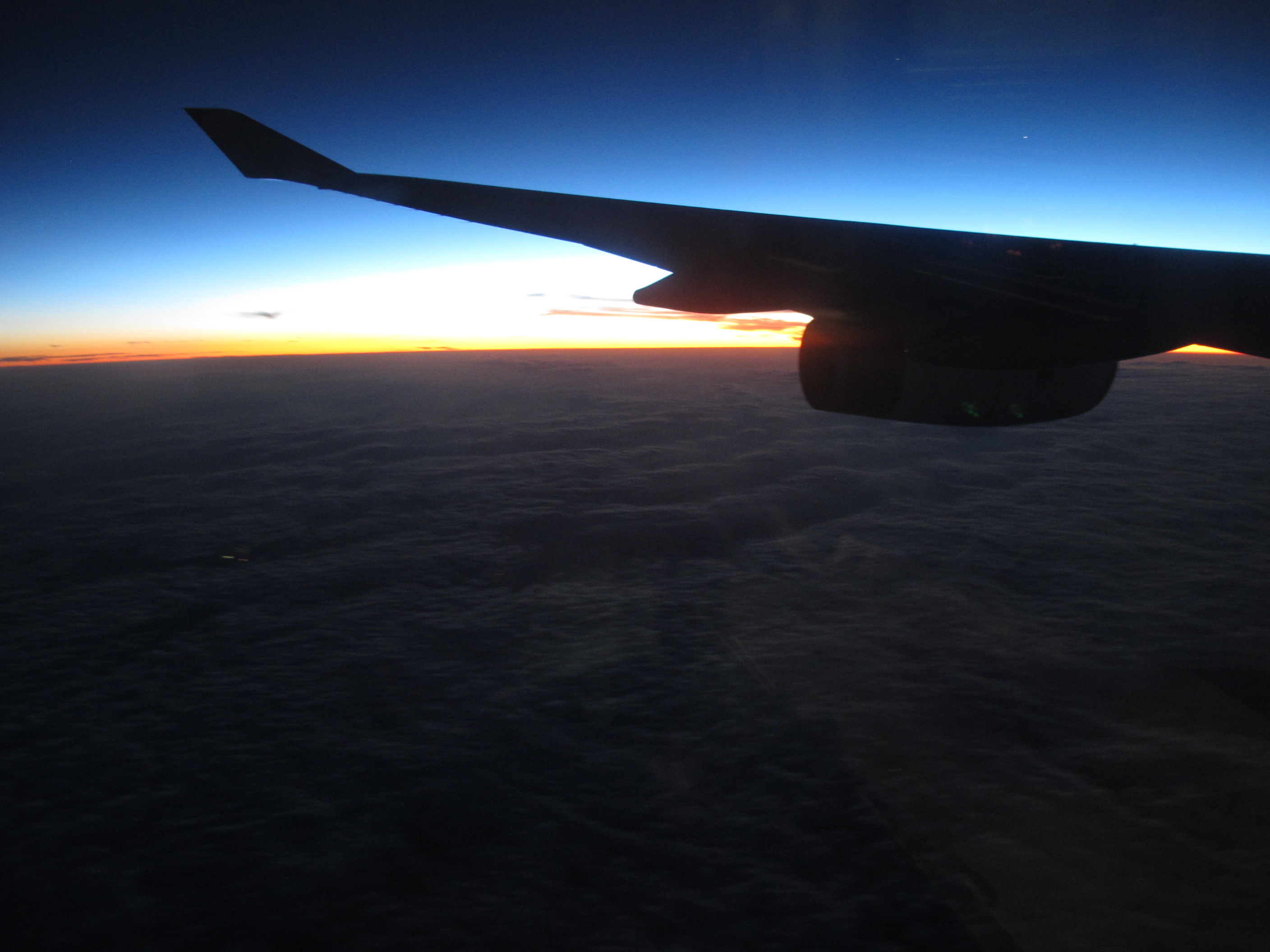
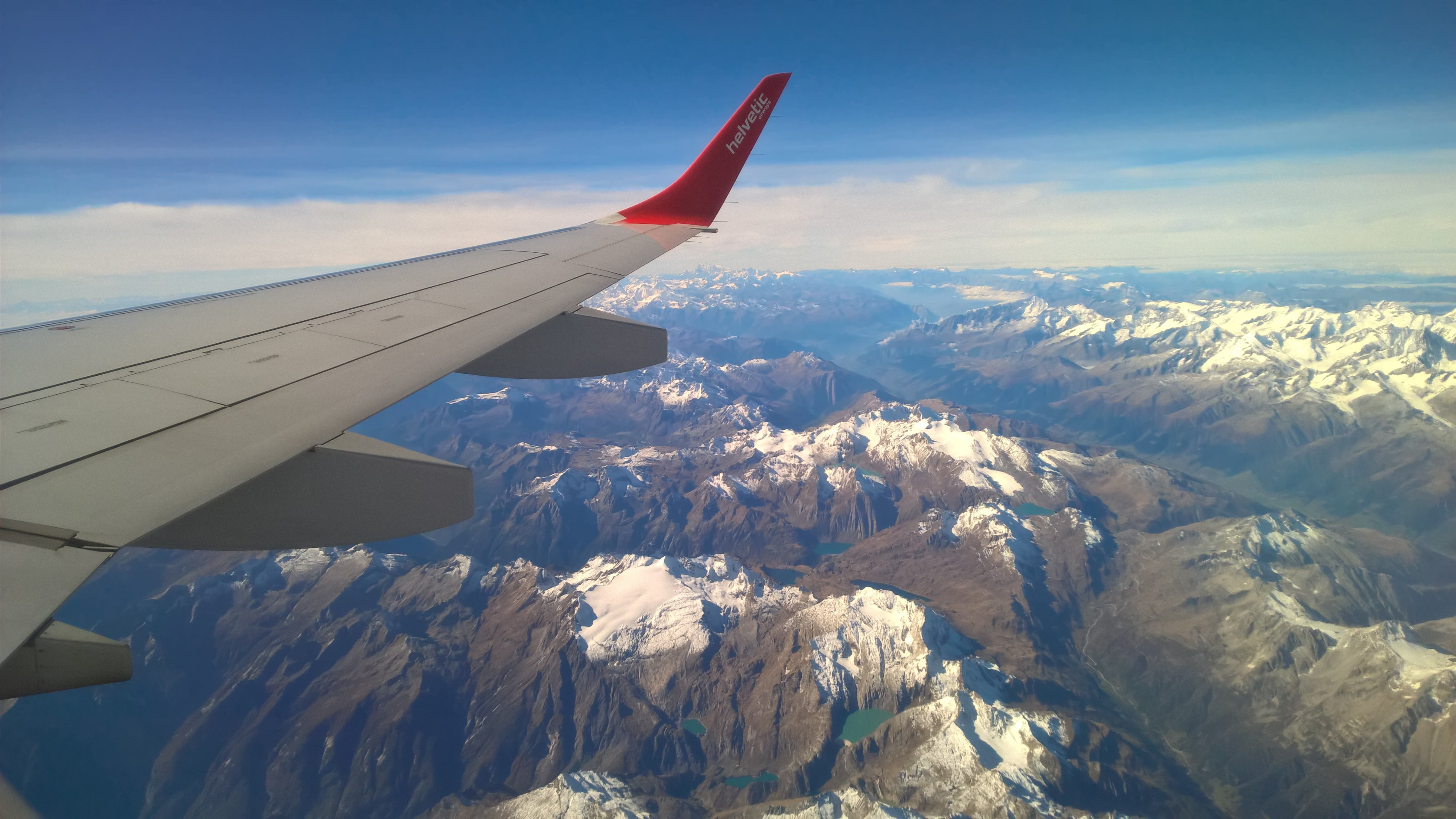
Tutorial 1.5: Measure Earth from an Airplane Window
The flagship Planet Ruler experience - accessible science with everyday tools.
This tutorial shows you how to measure Earth’s radius using nothing but your smartphone camera from an airplane window. It’s the perfect introduction to practical astronomy and demonstrates why Planet Ruler exists: to make planetary science accessible to everyone.
Prerequisites
A smartphone or camera with EXIF data
A window seat on a commercial flight
Basic knowledge of your flight altitude
30 minutes during flight + 15 minutes for analysis
Note
Perfect for: Students, teachers, curious travelers, anyone with a window seat and a sense of wonder! No special equipment needed.
The Science: Why This Works
From the ground, Earth’s horizon appears flat. But climb to 35,000 feet in an airplane, and you’ll see the horizon curve. This isn’t an optical illusion - you’re seeing Earth’s actual roundness.
The higher you go, the more curvature becomes visible. By measuring how much the horizon curves in your photo and knowing your altitude, you can reverse-engineer Earth’s radius.
Historical Context: Ancient Greek scientist Eratosthenes measured Earth’s circumference using a stick and the sun around 240 BCE. You’re doing something conceptually similar, but with modern tools that fit in your pocket!
Part 1: Taking Your Photo
Best Timing
When to photograph:
Altitude: 25,000 - 40,000 feet (typical commercial cruise altitude)
Timing: After reaching cruising altitude (~30-40 minutes into flight)
Weather: Clear day with visible horizon
Position: Window seat, preferably away from wing
What makes a good photo:
What to avoid:
Photography Tips
Step-by-step:

1. Wait for cruising altitude (seatbelt sign off)
2. Position yourself close to window, sitting upright
3. Keep phone/camera level (don't tilt up or down)
4. Turn OFF flash
5. Focus on the horizon line
6. Take 5-10 photos (increases your chances of a good one)
7. Note the time for altitude lookup later
Tip
Camera settings (if adjustable):
Use HDR mode if available
Capture at highest resolution
Turn off digital zoom
Let auto-exposure handle brightness
Part 3: Finding Your Altitude
You need to know your altitude when you took the photo. Here are four methods, from most to least accurate:
Method 1: FlightRadar24 (Recommended)
Real-time tracking:
1. Open FlightRadar24 app (free version works)
2. Search for your flight number
3. Note altitude when you took photos
4. Screenshot for reference
Post-flight lookup:
1. Visit flightradar24.com
2. Search your flight number and date
3. Use playback feature to find your photo timestamp
4. Read the altitude at that moment

Example: "AA1234 on Nov 4 at 14:23 UTC: 35,000 feet"
Method 2: In-Flight Display
Many aircraft show altitude on seatback screens or overhead displays.
1. Take photo of altitude display when you photograph horizon
2. Note the altitude in feet
3. Convert to meters: altitude_m = altitude_ft × 0.3048

Example: 35,000 feet = 10,668 meters
Method 3: Ask the Flight Crew
Flight attendants usually know the cruising altitude:
Polite question: "Hi! I'm doing a science project measuring Earth's
curvature. Could you tell me our cruising altitude today?"

Typical answer: "We're at 37,000 feet today."
Method 4: Estimate from Flight Type
If you can’t get exact altitude, use these typical values:
Flight Type |
Altitude (feet) |
Altitude (meters) |
|---|---|---|
Domestic short-haul |
30,000 - 35,000 |
9,144 - 10,668 |
Domestic long-haul |
35,000 - 39,000 |
10,668 - 11,887 |
International |
37,000 - 41,000 |
11,278 - 12,497 |
Warning
Altitude uncertainty of ±2,000 feet typically adds 5-10% error to your final radius measurement. Try to be as accurate as possible, but don’t worry if you can only estimate.
Part 4: Analysis with Planet Ruler
Now for the fun part - let’s measure Earth’s radius!
Zero-Config Workflow
Planet Ruler’s auto-config feature extracts camera parameters from your photo’s EXIF data:
import planet_ruler as pr
from planet_ruler.camera import create_config_from_image
from planet_ruler.uncertainty import calculate_parameter_uncertainty
from planet_ruler.fit import format_parameter_result

# Your airplane photo and altitude
photo_path = "airplane_horizon.jpg"  # Your actual photo filename
altitude_meters = 10668  # 35,000 feet = 10,668 meters

# Auto-detect camera from EXIF data
config = create_config_from_image(
    image_path=photo_path,
    altitude_m=altitude_meters,
    planet="earth",
    limits_preset="balanced",  # "tight", "balanced" (default), or "loose"
)

# See what was detected
print("Auto-detected camera:")
camera_info = config["camera_info"]
print(f"  Model: {camera_info.get('camera_model', 'Unknown')}")
f_mm = config["init_parameter_values"]["f"] * 1000
w_mm = config["init_parameter_values"]["w"] * 1000
print(f"  Focal length: {f_mm:.1f} mm")
print(f"  Sensor width: {w_mm:.1f} mm")

# Create observation
obs = pr.LimbObservation(photo_path, config)
Image Cropping (Optional)
Sometimes obstructions are unavoidable. If you end up with a photo that contains a window frame, airplane wing, or other object that either obscures the horizon directly or could confuse the fit, cropping is a great option. To get started, simply run the crop_image method. You’ll get a pop-up GUI containing your image where you can drag a rectangle that will contain the area you want to keep. Try to get as much of the horizon as you can while avoiding whatever is obscuring it.
obs.crop_image()
GUI controls
Crop Tool Controls:
Click & Drag     Select crop region
Scroll Wheel     Zoom in/out
+/- Keys         Zoom in/out
Esc              Clear selection

Buttons:
Crop & Save      Apply crop and save to disk
Crop (No Save)   Crop in-memory only
Clear Selection  Remove crop region
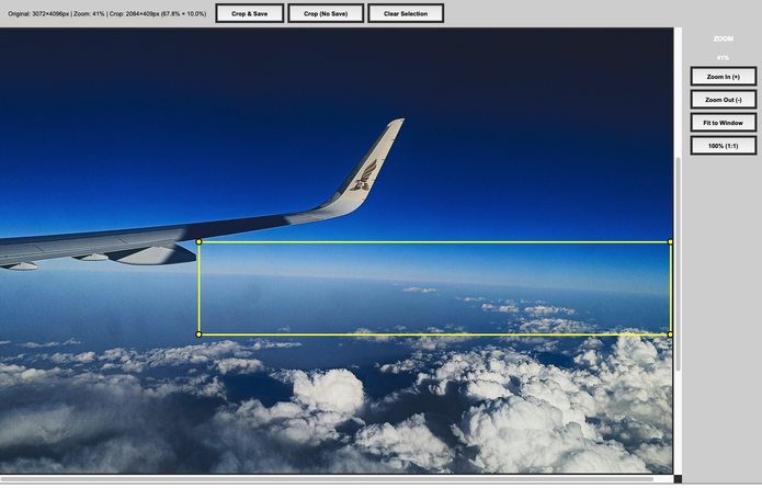
Drag the crop rectangle to select a region without obstuctions.
Note
Cropping the image implicitly changes the camera parameters (field of view, for one). Planet-ruler compensates for this by automatically re-scaling those parameters appropriately after you crop.
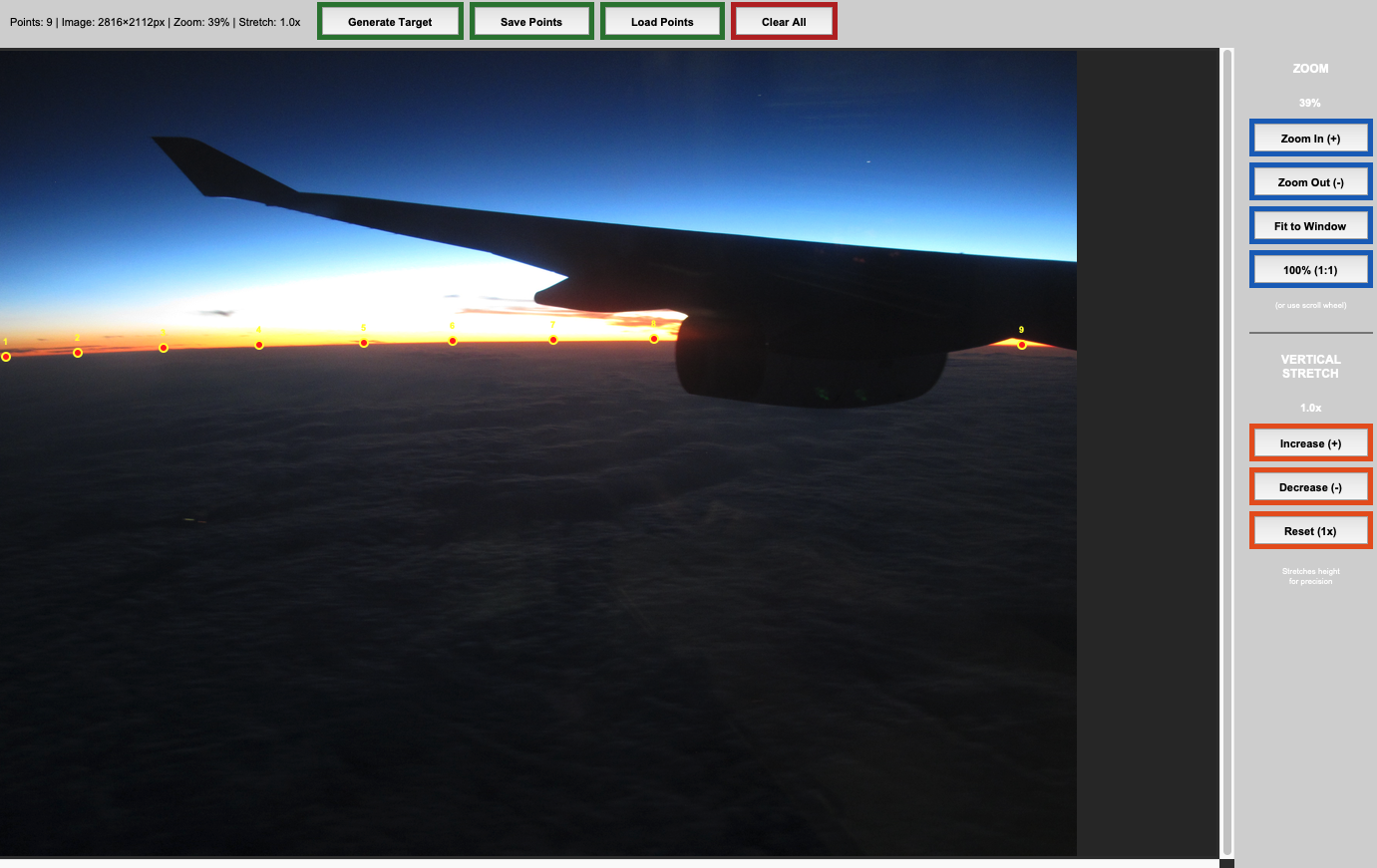
Horizon Detection
Use manual annotation for precise, user-controlled detection.
obs.detect_limb(detection_method="manual")
GUI controls
Crop Tool Controls:
Left Click Place horizon point
Right Click Remove previous point
Scroll Wheel Zoom in/out
+/- Keys Zoom in/out
Zoom Buttons:
Generate Target Save points to memory (ok to close window after)
Save Points Save points to disk for usage later
Load Points Load a previous set of points
Clear all Remove all points
Zoom In/Out Zoom in/out
Fit to Window Zoom to fit image vertically
100% (1:1) Zoom to full resolution
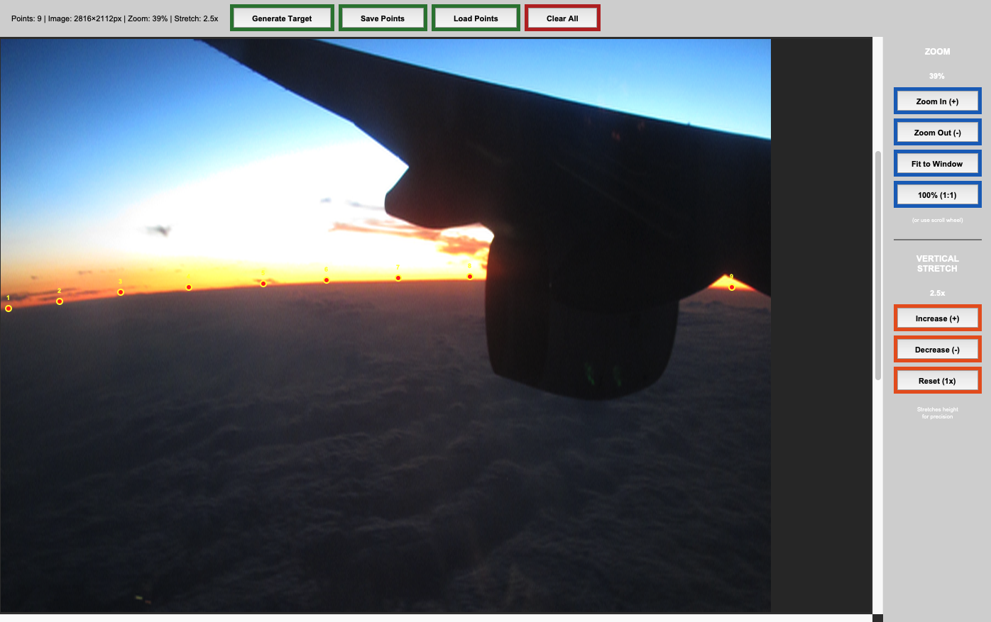
Vertical Stretch Buttons:
Increase Stretch image vertically (increases apparent curvature)
Decrease Relax image vertically (decreases apparent curvature)
Reset (1x) Restore original vertical ratio
Tip
Clicking strategy: Click 10-15 points spread evenly across the horizon. More points near areas of high curvature, fewer where horizon is straighter. Don’t be shy with the vertical stretch button – this makes it dramatically easier to see the curve and place points accurately.
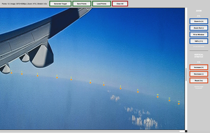
Annotating using a 4.5x vertical stretch.
Parameter Fitting
Now fit the planetary radius to match your detected horizon:
# Fit Earth's radius
print("\nFitting planetary parameters...")
obs.fit_arc(
    minimizer='differential-evolution',
    max_iter=1000,
    seed=42
)

print("✓ Fit completed!")
Results and Uncertainty
Extract your measurement with uncertainty quantification:
# Calculate radius with uncertainty
radius_result = calculate_parameter_uncertainty(
    obs, "r",
    scale_factor=1000,  # Convert meters to kilometers
    method='auto',
    confidence_level=0.68  # 1-sigma (68%)
)

# Display results
print("\n" + "="*50)
print("YOUR MEASUREMENT OF EARTH'S RADIUS")
print("="*50)
print(format_parameter_result(radius_result, "km"))

# Compare to known value
known_earth_radius = 6371.0  # km
error = abs(radius_result['value'] - known_earth_radius)
percent_error = 100 * error / known_earth_radius

print(f"\nKnown Earth radius: {known_earth_radius:.0f} km")
print(f"Your error: {error:.1f} km ({percent_error:.1f}%)")

if percent_error < 15:
    print("🎉 Excellent measurement!")
elif percent_error < 25:
    print("👍 Good measurement!")
else:
    print("📊 Try another photo for better accuracy")
Expected Output
Auto-detected camera:
  Apple iPhone 14 Pro
  Focal length: 24.0 mm
  Sensor width: 9.8 mm
  Field of view: 75.6°

Click points along the horizon curve...
✓ 22 points selected

Fitting planetary parameters...
✓ Fit completed!

==================================================
YOUR MEASUREMENT OF EARTH'S RADIUS
==================================================
r = 6234 ± 156 km

Known Earth radius: 6371 km
Your error: 137 km (2.2%)
🎉 Excellent measurement!
Part 5: Understanding Your Results
What to Expect
Typical Results:
Measured radius: 5,500 - 7,200 km
True Earth radius: 6,371 km
Typical error: 10-25%
Note
Even with 10-25% error, you’ve measured something the size of a planet using just your phone! That’s remarkable. Professional measurements use satellites and achieve centimeter precision, but your result is scientifically meaningful.
Sources of Error
Understanding why your measurement isn’t exactly 6,371 km:
1. Altitude Uncertainty (±5-10% effect)
In-flight displays are approximate
Barometric altitude vs. GPS altitude differ
Your location along the flight path varies
2. Camera Parameters (±5-10% effect)
EXIF focal length is approximate
Lens distortion (especially wide-angle phones)
Sensor size database contains estimates
Field-of-view calculation assumptions
3. Horizon Detection (±3-8% effect)
Manual clicking precision (±50-200 pixels)
Atmospheric haze obscures true horizon
Window clarity and cleanliness
Your hand stability when photographing
4. Atmospheric Refraction (±1-3% effect)
Light bends through atmosphere
Makes horizon appear slightly lower than geometric position
Not modeled in basic analysis
5. Earth’s Shape (±0-2% effect)
Earth is oblate (squashed): equatorial radius 6,378 km, polar radius 6,357 km
We assume a perfect sphere with mean radius 6,371 km
Your location matters slightly
Tip
The key insight: Despite these errors, you successfully measured a planetary-scale object! Understanding error sources is as educational as getting the “right” answer.
Improving Your Accuracy
Want better results? Try these techniques:
Multiple Measurements
# Analyze 3-5 photos from same flight
photos = ["photo1.jpg", "photo2.jpg", "photo3.jpg"]
results = []

for photo in photos:
    config = create_config_from_image(photo, altitude_m=10668, planet="earth")
    obs = pr.LimbObservation(photo, config)
    obs.detect_limb(detection_method="manual")
    obs.smooth_limb()
    obs.fit_arc(max_iter=1000)

    radius_result = calculate_parameter_uncertainty(
        obs, "r", scale_factor=1000, method='auto'
    )
    results.append(radius_result['value'])

# Average reduces random error
import numpy as np
print(f"Mean radius: {np.mean(results):.1f} km")
print(f"Std deviation: {np.std(results):.1f} km")
Better Altitude Data
GPS logger apps (more accurate than barometric)
Post-flight FlightRadar24 playback (most accurate)
Average altitude over 5-minute window
Optimal Photography
Clear day, minimal clouds
Clean windows (wipe if possible!)
Multiple exposures to ensure good quality
Steady hand or brace against window frame
Automated Detection
For more consistent results across multiple photos:
# Gradient-field optimization (no manual clicking, no detect_limb needed)
obs.fit_gradient(
    resolution_stages='auto',
    max_iter=800
)
Part 6: Educational Extensions
Class Projects
Individual Project:
Each student takes photos on a flight
Analyze individually with Planet Ruler
Compare results in class
Discuss error sources
Group Data Collection:
Pool results from entire class
Plot altitude vs. measurement accuracy
Identify patterns (time of day, location, weather)
Statistical analysis of combined data
Discussion Questions
Measurement Comparison
Who achieved the highest accuracy?
What made their photo better?
How did altitude affect results?
Error Analysis
Which error source was largest for your measurement?
How could we reduce each type of error?
What would professional scientists do differently?
Historical Context
How did Eratosthenes measure Earth 2,300 years ago?
How accurate was his measurement?
Why couldn’t ancient scientists use this airplane method?
Planetary Perspective
What does your measurement tell you about Earth’s size?
How does horizon curvature change with altitude?
Could you measure Mars this way if you were there?
Advanced Challenges
Challenge 1: Altitude vs. Accuracy
Hypothesis: Higher altitude gives more accurate measurements
1. Collect photos from flights at different altitudes
2. Process all with Planet Ruler
3. Plot: Altitude (x) vs. Measurement Error (y)
4. Is there a relationship?
Challenge 2: Earth’s Oblateness
Question: Can you detect that Earth is oblate (flattened at poles)?
1. Compare flights near equator (radius ~6,378 km)
   vs. near poles (radius ~6,357 km)
2. Does your measurement reflect this 21 km difference?
3. How much precision would you need?
Challenge 3: Weather Balloon
Extension: Measure from a weather balloon
1. Weather balloons reach ~100,000 feet
2. Much more curvature visible
3. Could achieve <5% accuracy
4. Great science fair project!
Part 7: Troubleshooting
Common Issues
“The detection isn’t finding my horizon”
Solution: Use manual annotation (method="manual"). You control every point, so it works with challenging images.
“My result is way off (like 100,000 km)”
Check: * Altitude is in meters, not feet (35,000 ft = 10,668 m) * Horizon is clearly visible in photo * You clicked along the actual horizon (not clouds or terrain)
“GUI window won’t open”
On Linux: sudo apt-get install python3-tk
On Mac/Windows: tkinter should be pre-installed
“Camera not in database”
Override with manual field-of-view:
# Use "loose" preset to give the optimizer more room when metadata is uncertain
config = create_config_from_image(
    photo_path,
    altitude_m=10668,
    planet="earth",
    limits_preset="loose",       # Wide search bounds
    param_tolerances={"f": 0.5}  # Extra slack on focal length
)
“My photo has the aircraft wing in it”
Use the crop tool to remove obstructions:
from planet_ruler.crop import crop_observation_image

# Interactive crop to remove wing
cropped_img, scaled_params, crop_bounds = crop_observation_image(
    image_path="airplane_photo.jpg",
    initial_parameters=config['observation']
)

# Instructions will appear:
# - Drag to select region without wing
# - Ensure full horizon arc is included
# - Click "Crop & Save" when done

# Save cropped image
cropped_img.save("airplane_photo_cropped.jpg")

# Update config with scaled parameters
config['observation'].update(scaled_params)

# Continue with normal workflow
obs = pr.LimbObservation("airplane_photo_cropped.jpg", config)
“The fitted arc curves the wrong way (arc sags downward instead of peaking upward)”
The optimizer occasionally locks onto a mirror-image solution where the predicted horizon curves in the opposite direction from the true limb. Planet Ruler includes a concavity penalty that prevents this by default, but if you see a clearly wrong fit you can try:
# Increase the penalty weight (default is 100) to push harder out of the wrong basin
obs.fit_arc(
    minimizer='differential-evolution',
    max_iter=1000,
    concavity_penalty_scale=500,
)

# Or re-run with a different random seed
obs.fit_arc(minimizer='differential-evolution', max_iter=1000, seed=99)
If you are photographing from an unusual angle where the horizon genuinely curves downward (rare outside of ISS or near-vertical imagery), disable the penalty:
obs.fit_arc(concavity_penalty=False)
“Result varies between photos”
Normal! Try: * Average multiple measurements * Use consistent horizon detection method * Ensure photos are all from similar altitude
Command Line Alternative
For batch processing or simpler workflow:
# One command to measure
planet-ruler measure \\
    --auto-config \\
    --altitude 10668 \\
    --planet earth \\
    --detection-method manual \\
    airplane_photo.jpg

# With custom field-of-view
planet-ruler measure \\
    --auto-config \\
    --altitude 10668 \\
    --field-of-view 75 \\
    airplane_photo.jpg
Next Steps
Continue Learning:
Try Examples for real spacecraft data
Explore API Reference for advanced techniques
Read about Quick Decision Tree to understand trade-offs
Share Your Science:
Post your result on social media with #PlanetRuler
Submit photos to the Planet Ruler community gallery (if available)
Help other students measure their data
Go Deeper:
Analyze multiple flights at different latitudes
Compare to other measurement methods (GPS, maps)
Build a class dataset and do statistical analysis
Write up results as a science fair project
Summary
Congratulations! You’ve measured Earth’s radius from an airplane window using nothing but your smartphone. You’re part of a scientific tradition going back millennia, but with tools that would have amazed ancient astronomers.
Key Takeaways:
Earth’s curvature is real and measurable from commercial flights
Everyday tools can do meaningful science
Understanding error is as important as the measurement itself
Experimental science is about process, not just “correct” answers
The Big Picture:
Even if your measurement had 20% error, you:
Engaged with the scientific method
Made a real observation of our planet
Quantified uncertainty in your data
Connected ancient science to modern tools
That’s what science is about. Well done!
Tip
For Educators: This tutorial aligns with NGSS standards for Earth and Space Sciences (ESS1), Engineering Design (ETS1), and Common Core Math standards for Geometry and Statistics. Consider using as a semester-long project with data collection, analysis, and presentation components.
Tutorial 2: Advanced Manual Annotation Techniques
Interactive GUI Features
The manual annotation interface provides several advanced features:
from planet_ruler.annotate import TkLimbAnnotator

# Load image for manual annotation
observation = obs.LimbObservation("complex_horizon_image.jpg", "config.yaml")

# Manual annotation opens interactive GUI with these features:
# - Left click: Add limb points
# - Right click: Remove nearby points
# - Mouse wheel: Zoom in/out
# - Arrow keys: Adjust image stretch/contrast
# - 'g': Generate target array from points
# - 's': Save points to JSON file
# - 'l': Load points from JSON file
# - ESC or 'q': Close window

observation.detect_limb(detection_method="manual")
Working with Difficult Images
For challenging images with clouds, terrain, or atmospheric effects:
# Use manual annotation with custom stretch for better visibility
observation = obs.LimbObservation("difficult_image.jpg", "config.yaml")

# The GUI allows real-time contrast adjustment:
# - Up arrow: Increase stretch (brighter)
# - Down arrow: Decrease stretch (darker)
# - Use zoom to focus on specific horizon sections

observation.detect_limb(detection_method="manual")
Saving and Loading Annotation Sessions
# Save your work during annotation:
# 1. Click points along the horizon
# 2. Press 's' to save points to JSON file
# 3. Continue later by pressing 'l' to load saved points

# You can also save/load programmatically:
from planet_ruler.annotate import TkLimbAnnotator

annotator = TkLimbAnnotator("image.jpg", initial_stretch=1.0)
# ... add points in GUI ...
annotator.save_points("my_horizon_points.json")

# Later session:
annotator.load_points("my_horizon_points.json")
Tutorial 2.5: Gradient-Field Automated Detection
This tutorial demonstrates the gradient-field detection method, which provides automated horizon detection without requiring ML dependencies or manual annotation.
When to Use Gradient-Field
Best for:
Clear, well-defined horizons with strong gradients
Atmospheric limbs without complex cloud structure
Batch processing multiple images
When PyTorch/ML dependencies are unavailable
Situations where reproducibility is critical
Not ideal for:
Horizons with multiple strong edges (use manual)
Very noisy or low-contrast images (use manual)
Complex cloud structures (use segmentation or manual)
Prerequisites
Python 3.10+ with Planet Ruler installed
Clear horizon photograph
Camera configuration file or auto-config
Step 1: Basic Gradient-Field Measurement
from planet_ruler.observation import LimbObservation
from planet_ruler.uncertainty import calculate_parameter_uncertainty

# Load observation
obs = LimbObservation(
    image_filepath="demo/images/ISS_Earth_horizon.jpg",
    fit_config="config/earth_iss_1.yaml"
)

# No detect_limb() call needed — fit_gradient works directly on the image
obs.fit_gradient(
    minimizer='dual-annealing',
    resolution_stages='auto',  # Multi-resolution optimization
    max_iter=3000
)

# Calculate uncertainty
result = calculate_parameter_uncertainty(
    obs, "r",
    scale_factor=1000,
    method='auto'
)

print(f"Radius: {result['value']:.1f} ± {result['uncertainty']:.1f} km")
obs.plot()
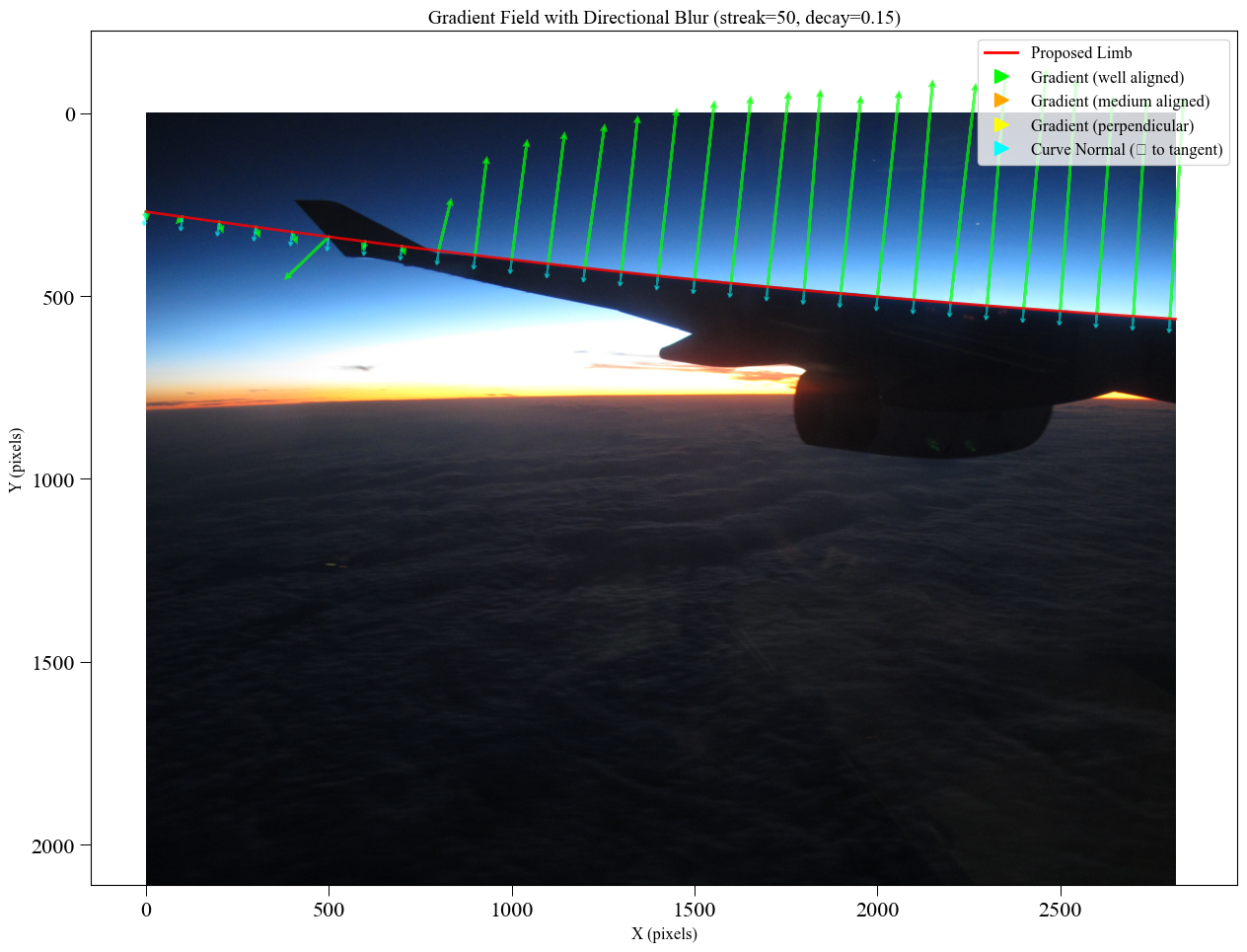
Step 2: Understanding Gradient-Field Parameters
The gradient-field method has several configurable parameters:
# Configure gradient-field fit
obs.fit_gradient(
    minimizer="dual-annealing",
    image_smoothing=2.0,
    kernel_smoothing=8.0,
    directional_smoothing=50,
    directional_decay_rate=0.10,  # Directional smoothing fall-off.
    prefer_direction="up",  # Hint: horizon is darker on top than bottom
)
Parameter Effects:
image_smoothing: Controls image smoothing _before_ gradient calculation. Helps with artifacts and other local minima.
Lower (0.5): Preserves fine details, more sensitive to noise
Higher (2.0): Smoother gradients, less noise sensitivity
kernel_smoothing: Controls image smoothing _after_ gradient calculation. Helps to homogenize noisy gradient directions.
Lower (1.0): Preserves fine details, more sensitive to noise
Higher (8.0): Smoother gradients, less noise sensitivity
directional_smoothing: Directional smoothing distance (along gradients). Helps avoid vanishing gradient in loss function.
Larger values (50): Casts a wide net to keep optimization from getting stuck. Can distort results depending on strength and how far the limb is from the edge of frame.
Smaller values (5): Slight speedup to optimization if already converging, but too low and fit may not converge to the true minimum.
directional_decay_rate: Rate of exponential decay in directional sampling
Larger values: Faster decay, emphasizes nearby pixels
Smaller values: Slower decay, includes more distant pixels
Step 3: Multi-Resolution Optimization
Gradient-field detection benefits greatly from multi-resolution optimization:
# Automatic multi-resolution (recommended)
obs.fit_gradient(
    minimizer="dual-annealing",
    resolution_stages='auto',  # Automatically generates stages
    max_iter=1000
)

# Manual multi-resolution configuration
obs.fit_gradient(
    minimizer="dual-annealing",
    resolution_stages=[4, 2, 1],  # Downsample factors: 4x → 2x → 1x
    max_iter=1000
)

# Single resolution (faster but may miss global optimum)
obs.fit_gradient(
    minimizer="dual-annealing",
    resolution_stages=None,  # No multi-resolution
    max_iter=1000
)
Multi-Resolution Benefits:
Avoids local minima by starting coarse
Progressively refines solution
More robust convergence
Slightly slower but much more reliable
Step 4: Choosing Minimizers for Gradient-Field
Different minimizers have different characteristics:
# Differential evolution: Best for complex problems
obs.fit_gradient(
    minimizer='differential-evolution',
    minimizer_preset='robust',     # "fast", "balanced", "robust", "super_robust"
    resolution_stages='auto',
    max_iter=1000,
    seed=42
)
# Pros: Most robust, provides population for uncertainty
# Cons: Slowest

# Dual annealing: Good balance
obs.fit_gradient(
    minimizer='dual-annealing',
    minimizer_preset='balanced',
    resolution_stages='auto',
    max_iter=1000,
    seed=42
)
# Pros: Fast, good global optimization
# Cons: No population (use Hessian for uncertainty)

# Basinhopping: Fastest
obs.fit_gradient(
    minimizer='basinhopping',
    minimizer_preset='fast',
    resolution_stages='auto',
    seed=42
)
# Pros: Fastest optimization
# Cons: May miss global optimum, use with multi-resolution
Step 5: Visualizing Gradient-Field Results
import matplotlib.pyplot as plt
import numpy as np
import planet_ruler.geometry

# Create comprehensive visualization
fig, axes = plt.subplots(2, 2, figsize=(14, 10))

# Original image
axes[0, 0].imshow(obs.image_data)
axes[0, 0].set_title("Original Image")
axes[0, 0].axis('off')

# Gradient field
obs.plot(gradient=True, ax=axes[0, 1], show=False)
axes[0, 1].set_title("Gradient Field")

# Detected limb overlay
axes[1, 0].imshow(obs.image_data)
x = np.arange(len(obs.features["limb"]))
axes[1, 0].plot(x, obs.features["limb"], 'r-', linewidth=2)
axes[1, 0].set_title("Detected Limb")
axes[1, 0].axis('off')

# Fit quality
x = np.arange(len(obs.features["limb"]))
axes[1, 1].plot(x, obs.features["limb"], 'b-',
                linewidth=2, label="Detected")

# Theoretical limb
final_params = obs.init_parameter_values.copy()
final_params.update(obs.best_parameters)
theoretical = planet_ruler.geometry.limb_arc(
    n_pix_x=len(obs.features["limb"]),
    n_pix_y=obs.image_data.shape[0],
    **final_params
)
axes[1, 1].plot(x, theoretical, 'r--',
                linewidth=2, label="Fitted model")
axes[1, 1].set_title("Fit Quality")
axes[1, 1].set_xlabel("Pixel X")
axes[1, 1].set_ylabel("Pixel Y")
axes[1, 1].legend()
axes[1, 1].grid(alpha=0.3)

plt.tight_layout()
plt.show()
Step 6: Batch Processing with Gradient-Field
The gradient-field method is ideal for batch processing:
from pathlib import Path
import pandas as pd

# Process multiple images
image_dir = Path("demo/images/")
image_files = list(image_dir.glob("*_horizon_*.jpg"))

results = []

for image_file in image_files:
    print(f"Processing {image_file.name}...")

    try:
        # Load and process
        obs = LimbObservation(
            str(image_file),
            "config/earth_iss_1.yaml"
        )

        # Automated fit directly to image gradients
        obs.fit_gradient(
            minimizer='dual-annealing',
            minimizer_preset='balanced',
            resolution_stages='auto',
            max_iter=500  # Reduce for speed
        )

        # Calculate uncertainty
        result = calculate_parameter_uncertainty(
            obs, "r", scale_factor=1000, method='auto'
        )

        results.append({
            'file': image_file.name,
            'radius_km': result['value'],
            'uncertainty_km': result['uncertainty'],
            'status': 'success'
        })

    except Exception as e:
        results.append({
            'file': image_file.name,
            'radius_km': None,
            'status': f'failed: {str(e)}'
        })

# Summary
df = pd.DataFrame(results)
print(df)

# Save results
df.to_csv("batch_results.csv", index=False)
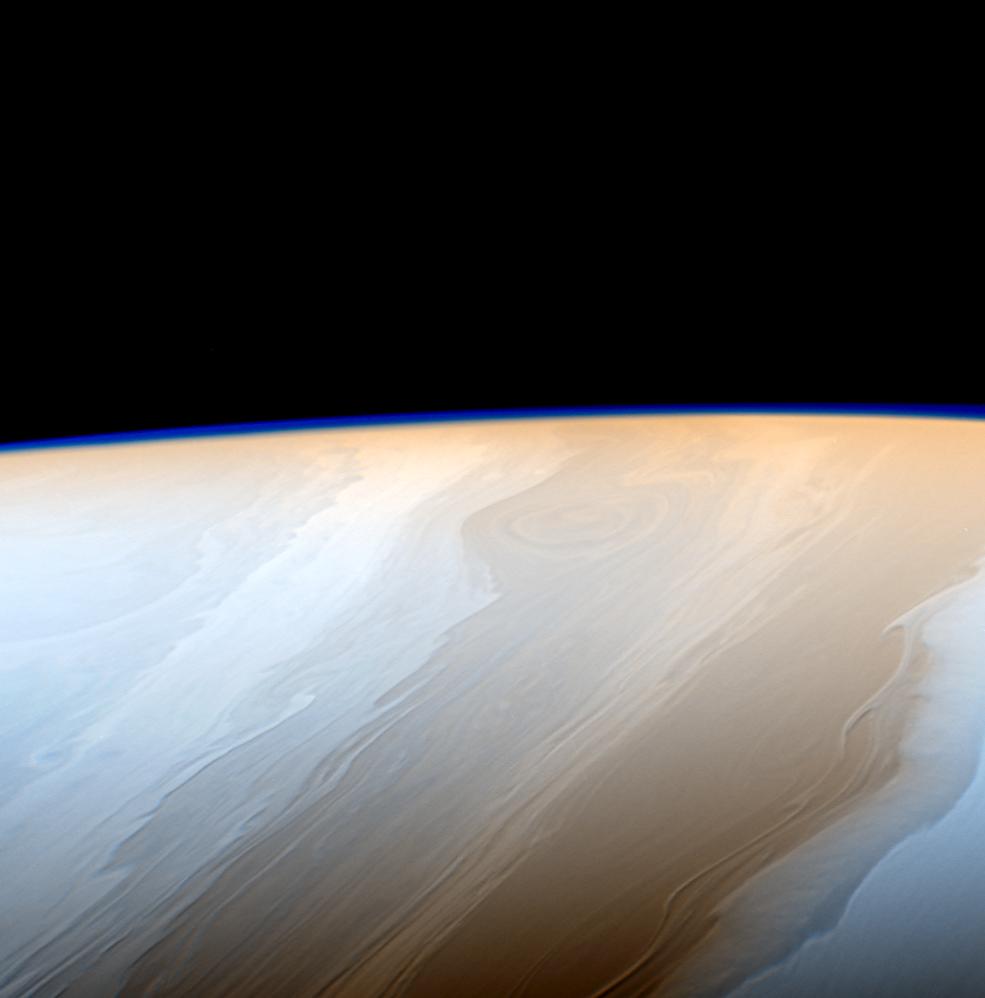
Tutorial 3: Multi-planetary Analysis (Manual Annotation)
Comparing Earth, Pluto, and Saturn with Precise Manual Selection
import pandas as pd
from planet_ruler.observation import LimbObservation
from planet_ruler.uncertainty import calculate_parameter_uncertainty

# Scenarios to analyze
scenarios = [
    ("Earth ISS", "config/earth_iss_1.yaml", "demo/images/earth_iss.jpg"),
    ("Pluto New Horizons", "config/pluto-new-horizons.yaml", "demo/images/pluto_nh.jpg"),
    ("Saturn Cassini", "config/saturn-cassini-1.yaml", "demo/images/saturn_cassini.jpg")
]

results = []

for name, config_path, image_path in scenarios:
    print(f"\nProcessing {name}...")

    # Load and process observation with manual annotation
    obs_obj = LimbObservation(image_path, config_path)

    print(f"  Opening manual annotation GUI for {name}...")
    print("  Instructions:")
    print("    - Click along the horizon to mark limb points")
    print("    - Use mouse wheel to zoom, arrows for contrast")
    print("    - Press 'g' to generate target, 's' to save, 'q' to close")

    # Use manual annotation (default, precise)
    obs_obj.detect_limb(detection_method="manual")
    method_used = "Manual Annotation"

    obs_obj.smooth_limb()
    obs_obj.fit_limb()

    # Calculate uncertainties
    radius_result = calculate_parameter_uncertainty(
        obs_obj, "r", scale_factor=1000, method="auto"
    )

    results.append({
        "Scenario": name,
        "Method": method_used,
        "Radius (km)": f"{radius_result['value']:.0f} ± {radius_result['uncertainty']:.0f}",
        "Uncertainty (km)": f"{radius_result['uncertainty']:.1f}",
        "Quality": "High (User-controlled precision)"
    })

# Display results table
df = pd.DataFrame(results)
print("\n" + "="*70)
print("MULTI-PLANETARY ANALYSIS RESULTS")
print("="*70)
print(df.to_string(index=False))
Tutorial 4: Detection Method Comparison
How to decide between Manual Annotation, Gradient-Field, and ML Segmentation
Planet Ruler offers three distinct methods for horizon detection, each with different trade-offs. This guide helps you choose the best method for your specific use case.
Quick Decision Tree
Method Overview
Comparison Table
Feature |
Manual Annotation |
Gradient-Field |
ML Segmentation |
Sagitta |
|---|---|---|---|---|
Setup Time |
Instant (built-in) |
Instant (built-in) |
5-10 min (first time model download) |
Instant (built-in) |
Processing Time |
30-120 sec (user-dependent) |
15-60 sec (automated) |
30-300 sec (model inference) |
<5 sec |
Dependencies |
None (tkinter only) |
None (scipy only) |
PyTorch + SAM (~2GB) |
None |
Memory Usage |
<100 MB |
<200 MB |
2-4 GB |
<100 MB |
Accuracy |
Highest (user-controlled) |
Good (clear horizons) |
Variable (depends on scene) |
Lower (best as first stage) |
Robustness |
Works everywhere |
Needs clear edges |
Handles complexity |
Needs detected limb |
Reproducibility |
Low (user variation) |
High (deterministic) |
High (deterministic) |
High (deterministic) |
Batch Processing |
Not practical |
Excellent |
Good (if GPU available) |
Excellent (as stage 1) |
Best Used As |
Standalone or stage 2 |
Standalone |
Standalone |
Stage 1 warm-start |
Method 1: Manual Annotation
Best for: First-time users, educational settings, challenging images
How It Works
Manual annotation uses an interactive GUI where you click points along the horizon.
It also lets you stretch the image vertically to exaggerate curvature and enhance accuracy.
Strengths:
Limitations:
When to Use
Use manual annotation when:
You’re analyzing 1-5 images
Image quality is poor (scratched windows, haze, clouds)
The horizon is ambiguous, obstructed, and/or complex
You want hands-on learning
You need to work immediately without dependencies
Example Usage
import planet_ruler as pr

# Load observation
obs = pr.LimbObservation("image.jpg", "config.yaml")

# Manual annotation (opens GUI)
obs.detect_limb(detection_method="manual")

# Fit annotated points
obs.fit_arc(max_iter=1000)
Tip
Best practices for clicking:
Cover as much horizontal area as you can
Click 10-20 points (more isn’t always better)
Concentrate points where curvature is higher
Zoom in or use Stretch for precision
Right click (undo) or clear points to undo bad placements
Visual Examples
Raw image |
Human-Annotated |
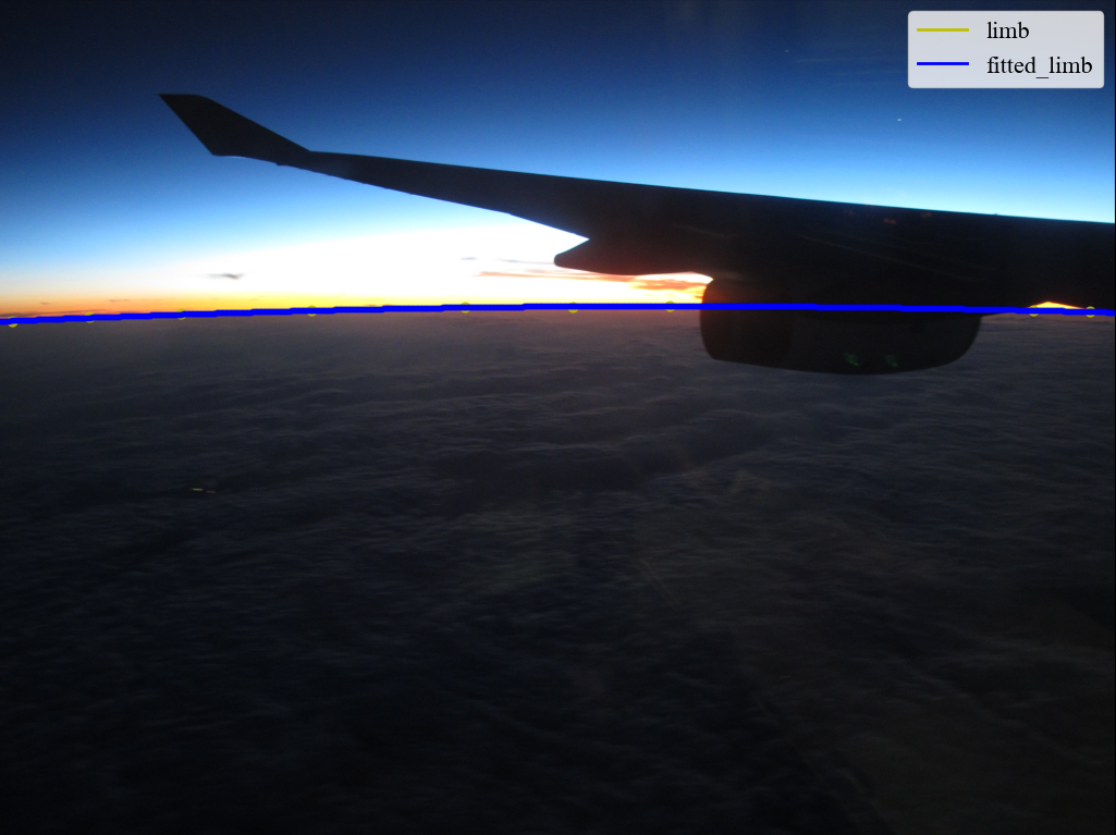
Planet radius fitted |
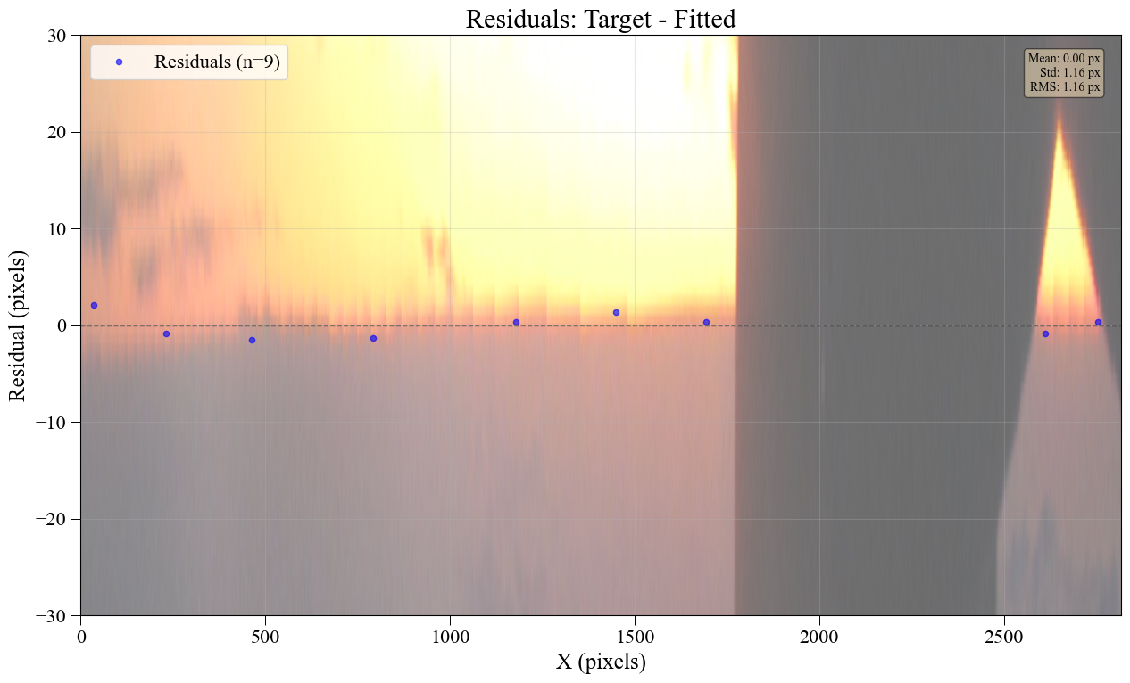
Fit residuals |
Example 1: Clear Horizon
Manual annotation goes quickly with clear horizons.
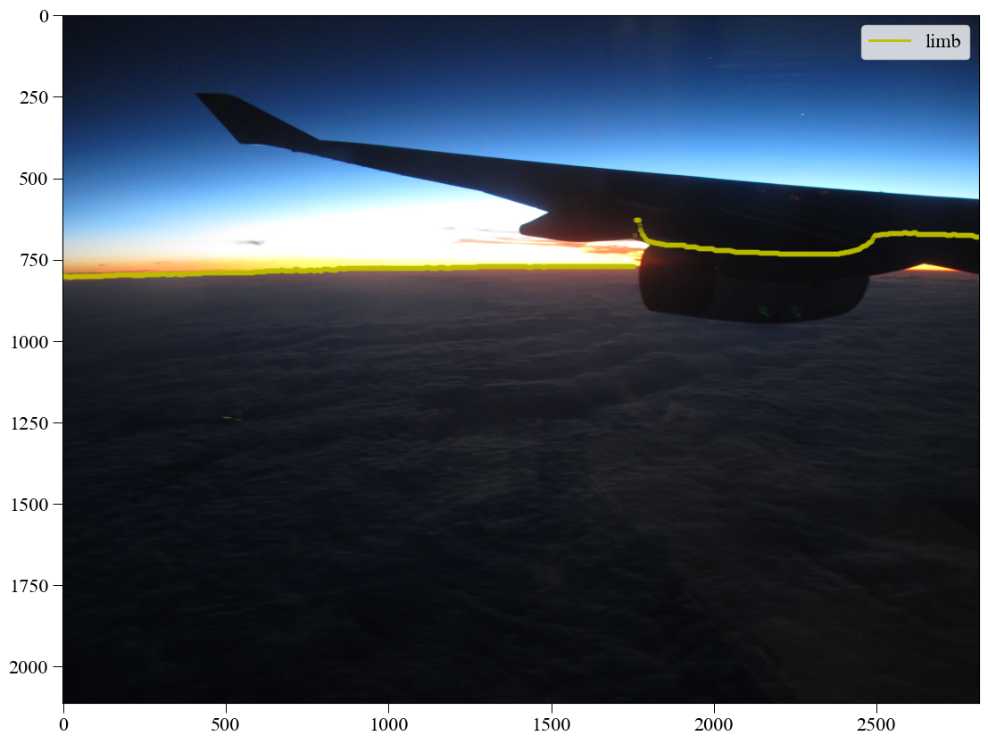
Example 2: Obstructions
User can avoid obstructions that can be tricky for automated methods.
Example 3: Complex Scene
Anything besides a human would struggle with this.
Method 2: Gradient-Field Detection
Best for: Batch processing, clear horizons, reproducible workflows
How It Works
Gradient-field detection skips explicit horizon detection entirely. Instead, it optimizes parameters directly on the image using brightness gradients perpendicular to the predicted horizon.
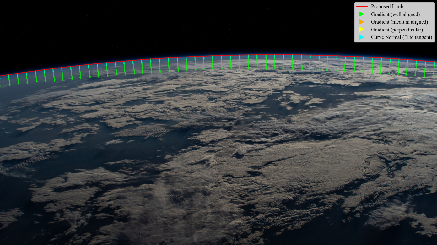
A ‘good’ horizon is one with high brightness gradient (flux) traversing its boundary.
The method uses multi-resolution optimization (coarse → fine) to avoid local minima.
Strengths:
Limitations:
When to Use
Use gradient-field when:
You’re batch processing many images (10+)
Horizons are sharp and well-defined
You want reproducible results
You don’t have time for manual annotation
You want lightweight processing (no GPU needed)
Images are clean with minimal obstruction
Example Usage
import planet_ruler as pr

# Load observation
obs = pr.LimbObservation("image.jpg", "config.yaml")

# Gradient-field optimization (no detection step!)
obs.fit_gradient(
    resolution_stages='auto',      # Multi-resolution: 0.25 → 0.5 → 1.0
    image_smoothing=2.0,           # Remove high-freq artifacts
    kernel_smoothing=8.0,          # Smooth gradient field
    minimizer='dual-annealing',
    minimizer_preset='balanced',
    max_iter=1000
)

# Note: No detect_limb() call needed!
Tip
Tuning parameters:
Increase
image_smoothing(2.0 → 4.0) for noisy imagesIncrease
kernel_smoothing(8.0 → 16.0) for hazy horizonsUse
prefer_direction="up"if above the horizon is darker than belowMore resolution stages (e.g., [8,4,2,1]) or
minimizer_preset='robust'for difficult cases
Visual Examples
Inside the Process
Raw image |
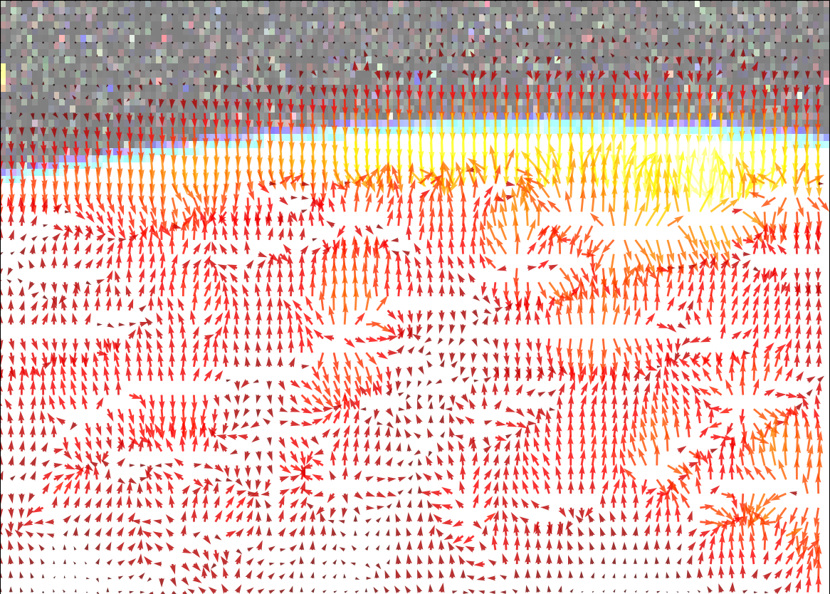
Gradient field |
Planet radius fitted |
“Flux” through fitted radius |
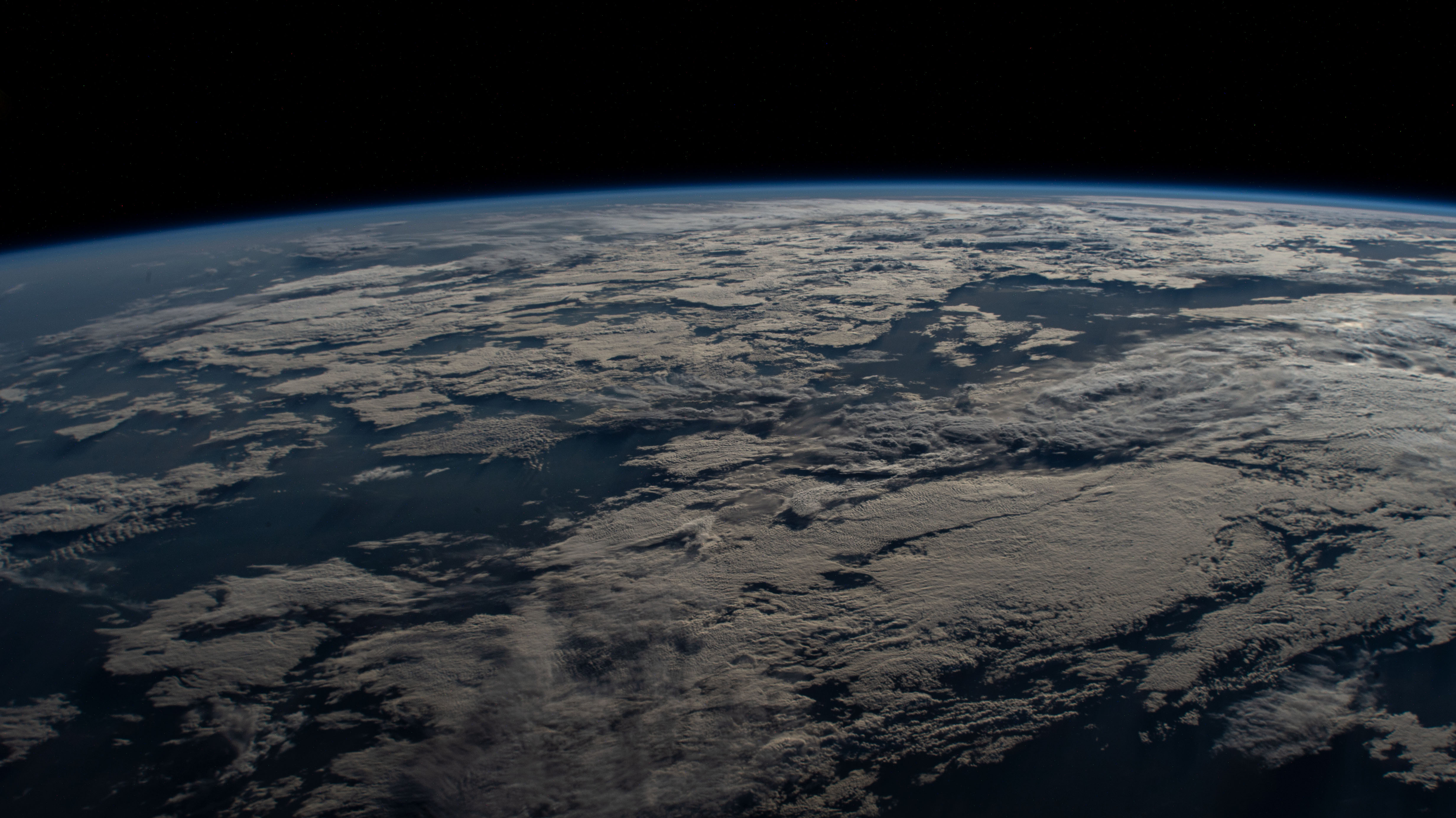
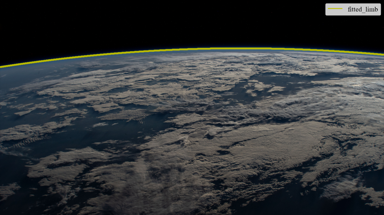
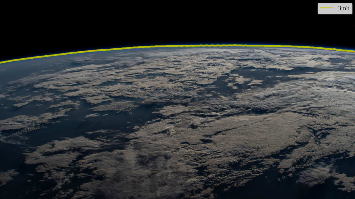
Example 1: ISS Earth Photo
Caption: Gradient-field works perfectly on clean spacecraft imagery.
Example 2: New Horizons Photo
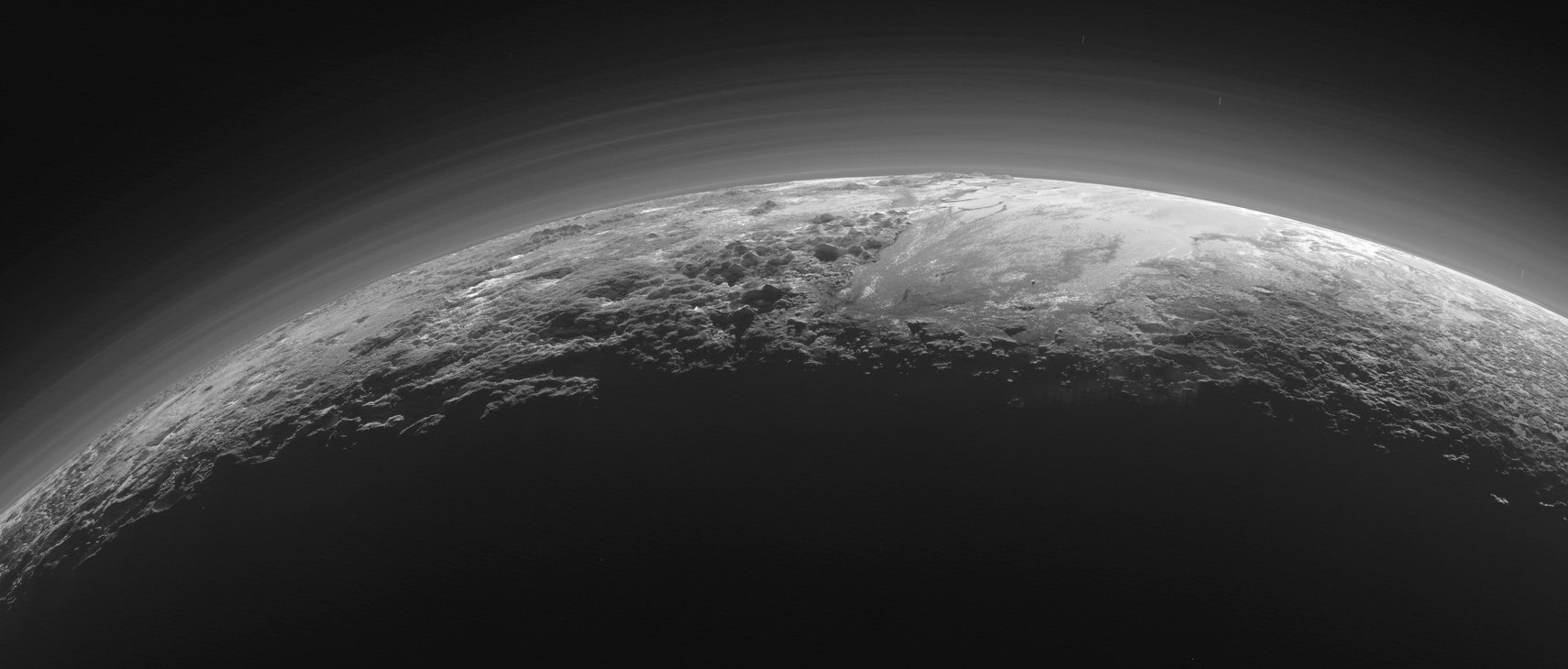
Caption: Hazy atmospheric boundary detected accurately. Multi-resolution helps.
Example 3: Failure Case
In this case it may have been better to go with manual annotation…
Performance Notes
Typical timing (Intel i7, 2000x1500 image):

Resolution stages [4, 2, 1]:
- Stage 1 (500x375):     8 sec
- Stage 2 (1000x750):   12 sec
- Stage 3 (2000x1500):  20 sec
Total: ~40 seconds

Memory usage: <200 MB
Method 3: ML Segmentation
Best for: Complex scenes, when you have GPU + PyTorch installed
How It Works
ML segmentation such as Meta’s Segment Anything Model (SAM) can be used to automatically detect the planetary body. In automatic mode (interactive=False), the model assumes the two largest masks are the planet and sky and labels their boundary as the horizon.
|
Original |
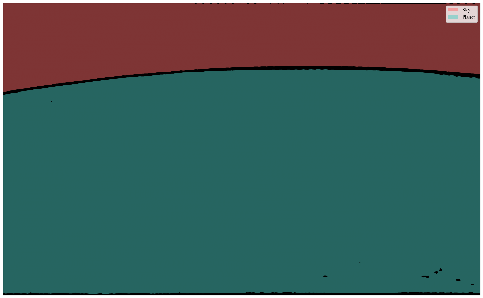
Segmented image |
Detected limb |
When set to interactive, however, the user is allowed to validate which masks belong to the sky and planet (or which to exclude) before the horizon is determined. This can help with obscuring objects like airplane wings or clouds. Note this method still isn’t foolproof – stay tuned for updates!
|
Original |
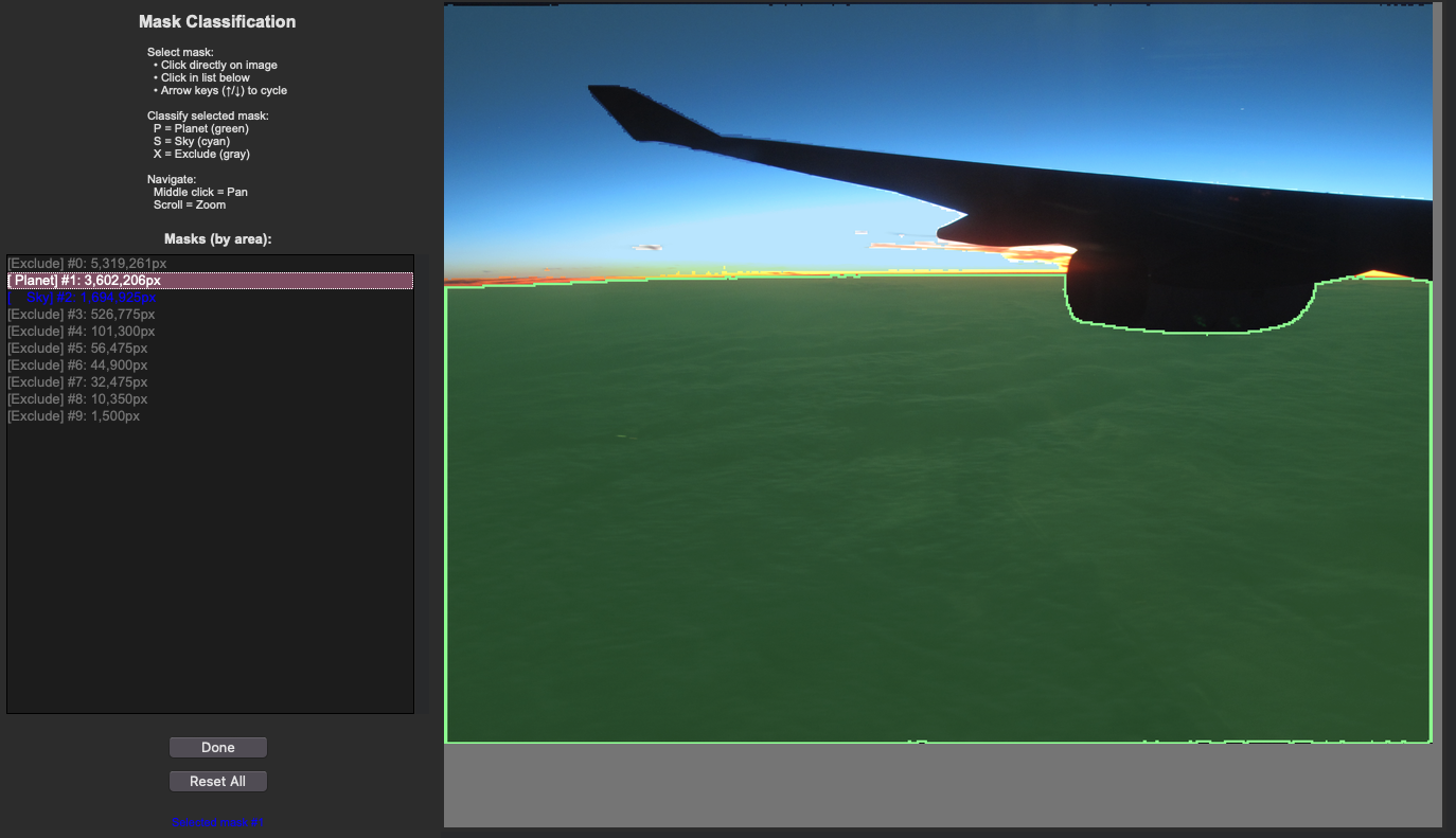
User Mask Annotation |
Detected limb |
Strengths:
Limitations:
When to Use
Use ML segmentation when:
You have PyTorch and GPU available
Scenes are complex (clouds, haze, terrain)
You want to avoid manual clicking
You’re willing to accept occasional failures
Images have clear color/brightness differences at horizon
You’re processing a moderate number of images (5-50)
Example Usage
import planet_ruler as pr

# First time only: model will auto-download (~2GB)
# This takes 5-10 minutes on first use

# Load observation
obs = pr.LimbObservation("image.jpg", "config.yaml")

# ML segmentation
obs.detect_limb(detection_method="segmentation")

# Always inspect the result!
obs.plot()

# If detection looks good, proceed
obs.fit_arc(max_iter=1000)
Warning
Always visually inspect ML segmentation results before fitting! The model can occasionally misidentify features as the horizon. If the detection looks wrong, use interactive mode or manual annotation instead.
Installation
# Install PyTorch (CPU version)
pip install torch torchvision --index-url https://download.pytorch.org/whl/cpu

# Install Segment Anything Model
pip install segment-anything

# For GPU support (faster, requires CUDA)
pip install torch torchvision --index-url https://download.pytorch.org/whl/cu118
Method 4: Sagitta (Arc-Height) Estimation
Best for: Quick radius estimates, warm-starting a subsequent arc fit
How It Works
The sagitta method estimates the planetary radius directly from the vertical “sag” of the horizon arc — the pixel distance between the highest and lowest points of the detected limb. It runs a fast 2-D optimizer over curvature and tilt and does not need differential evolution, making it much faster than a full arc fit.
Because it updates the parameter bounds automatically, it is especially useful
as a first stage that narrows the search space for a subsequent
fit_arc or fit_gradient call.
Strengths:
Limitations:
detect_limb() firstWhen to Use
Use the sagitta method when:
You want a fast sanity-check radius before committing to a full fit
You want to warm-start a slower arc or gradient-field optimization
You are processing many images and speed is critical
Example Usage
import planet_ruler as pr

obs = pr.LimbObservation("image.jpg", "config.yaml")
obs.detect_limb(detection_method="manual")

# Stand-alone sagitta estimate (fast)
obs.fit_sagitta()
print(f"Quick radius estimate: {obs.best_parameters['r']/1000:.0f} km")

# Or chain sagitta → arc for speed + accuracy (recommended combo)
obs.fit_limb(stages=[
    {"method": "sagitta"},
    {"method": "arc", "minimizer": "differential-evolution",
     "minimizer_preset": "balanced"},
])
print(f"Final radius: {obs.best_parameters['r']/1000:.0f} km")
Tip
The sagitta → arc chain is the recommended default workflow for manual annotation in 2.0. Sagitta quickly finds a good starting radius and tightens the parameter bounds; the arc fitter then refines it precisely.
Combining Methods
Best Practices Workflow
For critical measurements, use multiple methods and compare:
import planet_ruler as pr
from planet_ruler.uncertainty import calculate_parameter_uncertainty

results = {}

# Manual annotation → arc fit
print("\nTrying manual method...")
obs = pr.LimbObservation("image.jpg", "config.yaml")
obs.detect_limb(detection_method='manual')
obs.fit_arc()
results['manual'] = obs

# Gradient-field: no detection step needed
print("\nTrying gradient method...")
obs = pr.LimbObservation("image.jpg", "config.yaml")
obs.fit_gradient(resolution_stages='auto')
results['gradient'] = obs

# ML segmentation → arc fit
print("\nTrying ML segmentation method...")
obs = pr.LimbObservation("image.jpg", "config.yaml")
obs.detect_limb(detection_method='segmentation')
obs.fit_arc()
results['ml'] = obs

# Compare results
print("\nMethod comparison:")
radii = {}
for name, obs in results.items():
    radius_result = calculate_parameter_uncertainty(
        obs, "r", scale_factor=1000, method='auto'
    )
    radii[name] = radius_result['value']
    print(f"  {name}: {radius_result['value']:.1f} km")

# Check consistency
import numpy as np
values = list(radii.values())
print(f"\nSpread: {np.max(values) - np.min(values):.1f} km")
print(f"Mean: {np.mean(values):.1f} km")
print(f"Std: {np.std(values):.1f} km")
Troubleshooting Decision Guide
If Your Results Look Wrong
Problem: Manual annotation gives inconsistent results
Solution: Click points with more care
Solution: Use zoom/stretch features for precision
Solution: Try gradient-field for comparison
Problem: Gradient-field result is way off
Check: Is horizon clearly visible and sharp?
Check: Are there clouds or haze at horizon level?
Solution: Increase smoothing parameters (image_smoothing=4.0)
Solution: Add more resolution stages [8,4,2,1]
Fallback: Use manual annotation
Problem: ML segmentation detects wrong features
Check: Visually inspect with
obs.plot()before fittingSolution: Try interactive mode to refine masks
Solution: Increase smoothing after detection
Fallback: Use manual annotation (always reliable)
Summary
Choose Manual Annotation if:
You want maximum accuracy
You’re analyzing 1-10 images
You’re teaching or learning
Image quality is poor
You can spare 1-2 minutes per image
Choose Gradient-Field if:
You’re batch processing many images
Horizons are clean and sharp
You want reproducible results
You don’t have GPU/PyTorch
Speed is important
Choose ML Segmentation if:
You have PyTorch + GPU installed
Scenes are complex but horizon is visible
You want to experiment with AI methods
You’re willing to visually inspect results
You have time for model download (first time)
Use Sagitta as Stage 1 when:
You want a fast warm-start before a slower arc fit
You need a quick sanity-check radius estimate
You are batch processing and want to reduce full-fit time
When in doubt: Start with manual annotation followed by a sagitta → arc staged
fit (obs.fit_limb(stages=[{"method": "sagitta"}, {"method": "arc"}])).
This is the recommended default workflow in 2.0.
Next Steps
Try Prerequisites for a complete walkthrough with manual annotation
See When to Use Gradient-Field for gradient-field examples
Check Examples for real-world comparisons
Read API Reference for advanced configuration options
Installation and Setup
Basic Installation
Planet Ruler works immediately after installation with no additional dependencies:
# Essential: Install Planet Ruler (manual annotation works immediately)
python -m pip install planet-ruler
Verification Test
# Test basic Planet Ruler functionality
import planet_ruler.observation as obs
import planet_ruler.geometry as geom

# Test geometry functions
horizon_dist = geom.horizon_distance(r=6371000, h=400000)
print(f"✓ Planet Ruler installed - ISS horizon distance: {horizon_dist/1000:.1f} km")

# Test manual annotation interface
try:
    from planet_ruler.annotate import TkLimbAnnotator
    print("✓ Manual annotation GUI available")
except ImportError as e:
    print(f"⚠ GUI not available: {e}")
Optional: Advanced Detection Methods
For automatic detection methods, install additional dependencies:
# Optional: AI segmentation support (requires PyTorch + Segment Anything)
python -m pip install segment-anything torch torchvision

# Optional: GPU support for faster AI processing
python -m pip install torch torchvision --index-url https://download.pytorch.org/whl/cu118
Testing Optional Dependencies
# Test AI segmentation installation (optional)
try:
    from planet_ruler.image import MaskSegmenter
    from segment_anything import sam_model_registry
    print("✓ AI segmentation available")
except ImportError as e:
    print(f"⚠ AI segmentation not available: {e}")
    print("Install with: pip install segment-anything torch")
Troubleshooting
Common issues and solutions:
Manual annotation GUI not opening
# Ensure tkinter is installed (usually included with Python)
python -m tkinter  # Should open a test window
“No module named ‘segment_anything’” (for AI segmentation only)
python -m pip install segment-anything torch
Performance tips for manual annotation
# For large images, consider downsampling for easier annotation:
from PIL import Image

# Resize image before annotation if needed
img = Image.open("large_image.jpg")
img_resized = img.resize((img.width//2, img.height//2))
img_resized.save("resized_for_annotation.jpg")
Next Steps
Review Installation for detailed setup instructions
Explore Examples section for real mission data with manual annotation
Check API Reference documentation for all detection method parameters
See Performance Benchmarks for performance analysis across detection methods