How to decide between Manual Annotation, Gradient-Field, and ML Segmentation

Planet Ruler offers three distinct methods for horizon detection, each with different trade-offs. This guide helps you choose the best method for your specific use case.

Quick Decision Tree

flowchart TD Start([Start]) --> Q1{Is horizon<br/>obstructed?} Q1 -->|YES| Q2{GPU Available?} Q1 -->|NO| Q3{Smooth horizon line?} Q2 -->|YES| ML1[ML Segmentation:<br/>Interactive Mode] Q2 -->|NO| Manual1[Manual Annotation:<br/>Click around obstructions] Q3 -->|YES| Q4{Prefer automated?} Q3 -->|NO| Q2 Q4 -->|YES| Q5{GPU Available?} Q4 -->|NO| Manual2[Manual Annotation:<br/>Fast & foolproof] Q5 -->|YES| ML2[ML Segmentation:<br/>Automatic mode] Q5 -->|NO| Gradient1[Gradient-Field:<br/>Fast, lightweight] style Manual1 fill:#90EE90 style Manual2 fill:#90EE90 style Gradient1 fill:#87CEEB style ML1 fill:#FFB6C1 style ML2 fill:#FFB6C1

Method Overview

Comparison Table

Detection & Fitting Method Comparison

Feature	Manual Annotation	Gradient-Field	ML Segmentation	Sagitta
Setup Time	Instant (built-in)	Instant (built-in)	5-10 min (first time model download)	Instant (built-in)
Processing Time	30-120 sec (user-dependent)	15-60 sec (automated)	30-300 sec (model inference)	<5 sec
Dependencies	None (tkinter only)	None (scipy only)	PyTorch + SAM (~2GB)	None
Memory Usage	<100 MB	<200 MB	2-4 GB	<100 MB
Accuracy	Highest (user-controlled)	Good (clear horizons)	Variable (depends on scene)	Lower (best as first stage)
Robustness	Works everywhere	Needs clear edges	Handles complexity	Needs detected limb
Reproducibility	Low (user variation)	High (deterministic)	High (deterministic)	High (deterministic)
Batch Processing	Not practical	Excellent	Good (if GPU available)	Excellent (as stage 1)
Best Used As	Standalone or stage 2	Standalone	Standalone	Stage 1 warm-start

Method 1: Manual Annotation

Best for: First-time users, educational settings, challenging images

How It Works

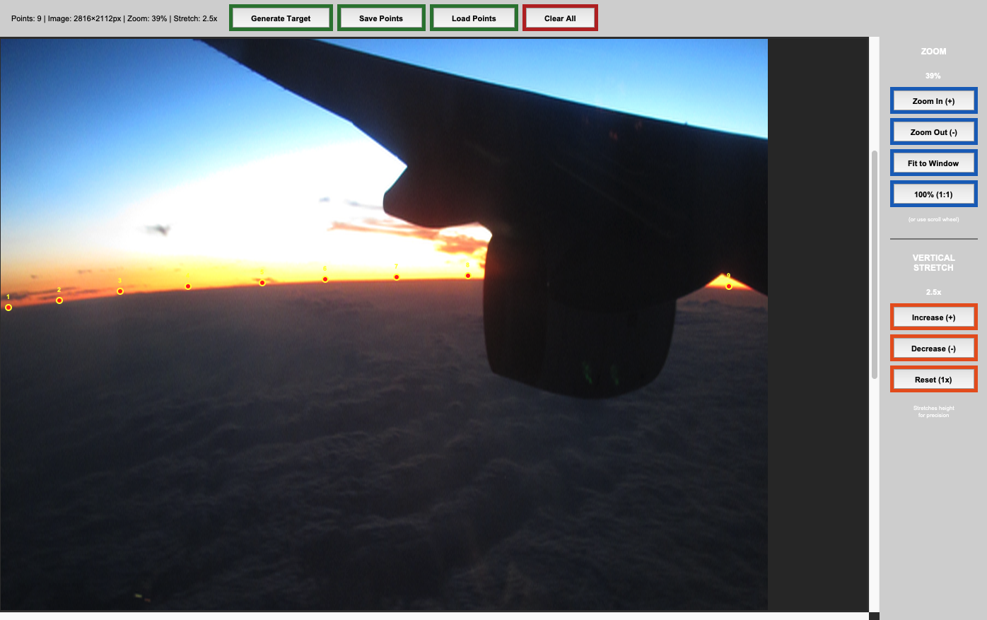
Manual annotation uses an interactive GUI where you click points along the horizon.

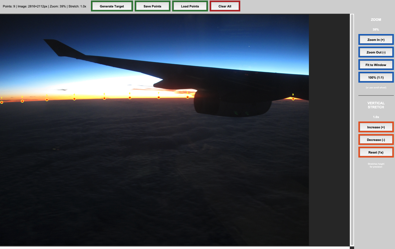
It also lets you stretch the image vertically to exaggerate curvature and enhance accuracy.

Strengths:

✅ Universal applicability - Works with any image that has a visible horizon

✅ No dependencies - Works immediately after installing Planet Ruler

✅ Educational - Students learn by actively identifying the horizon

✅ Handles complexity - Clouds, haze, wing, terrain? You decide what’s horizon

Limitations:

❌ User-dependent - Different people get slightly different results

❌ Time-consuming - Takes 30-120 seconds per image

❌ Not batch-friendly - Must manually process each image

❌ Requires practice - Takes a few tries to get good at point placement

When to Use

Use manual annotation when:

• You’re analyzing 1-5 images

• Image quality is poor (scratched windows, haze, clouds)

• The horizon is ambiguous, obstructed, and/or complex

• You want hands-on learning

• You need to work immediately without dependencies

Example Usage

import planet_ruler as pr

# Load observation
obs = pr.LimbObservation("image.jpg", "config.yaml")

# Manual annotation (opens GUI)
obs.detect_limb(detection_method="manual")

# Fit annotated points
obs.fit_arc(max_iter=1000)

Tip

Best practices for clicking:

• Cover as much horizontal area as you can

• Click 10-20 points (more isn’t always better)

• Concentrate points where curvature is higher

• Zoom in or use Stretch for precision

• Right click (undo) or clear points to undo bad placements

Visual Examples

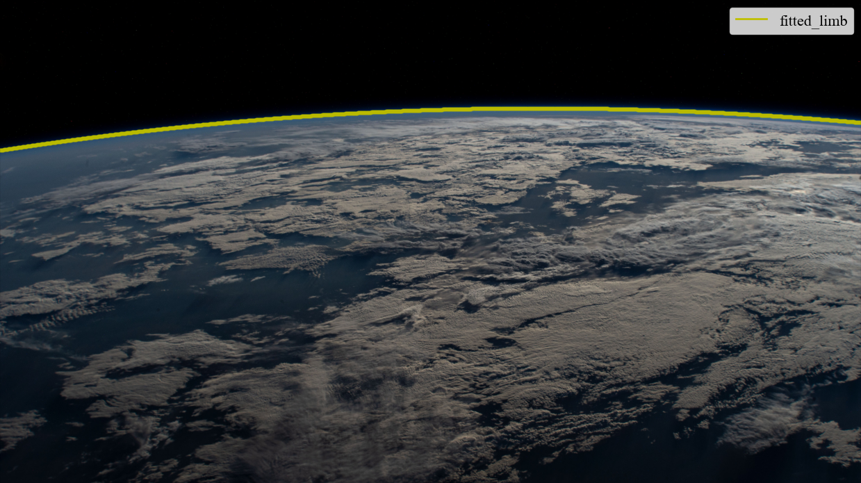
Raw image	Human-Annotated
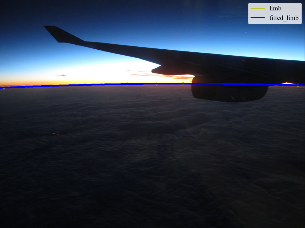
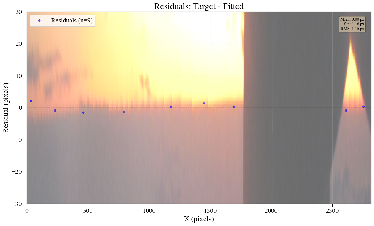
Planet radius fitted	Fit residuals

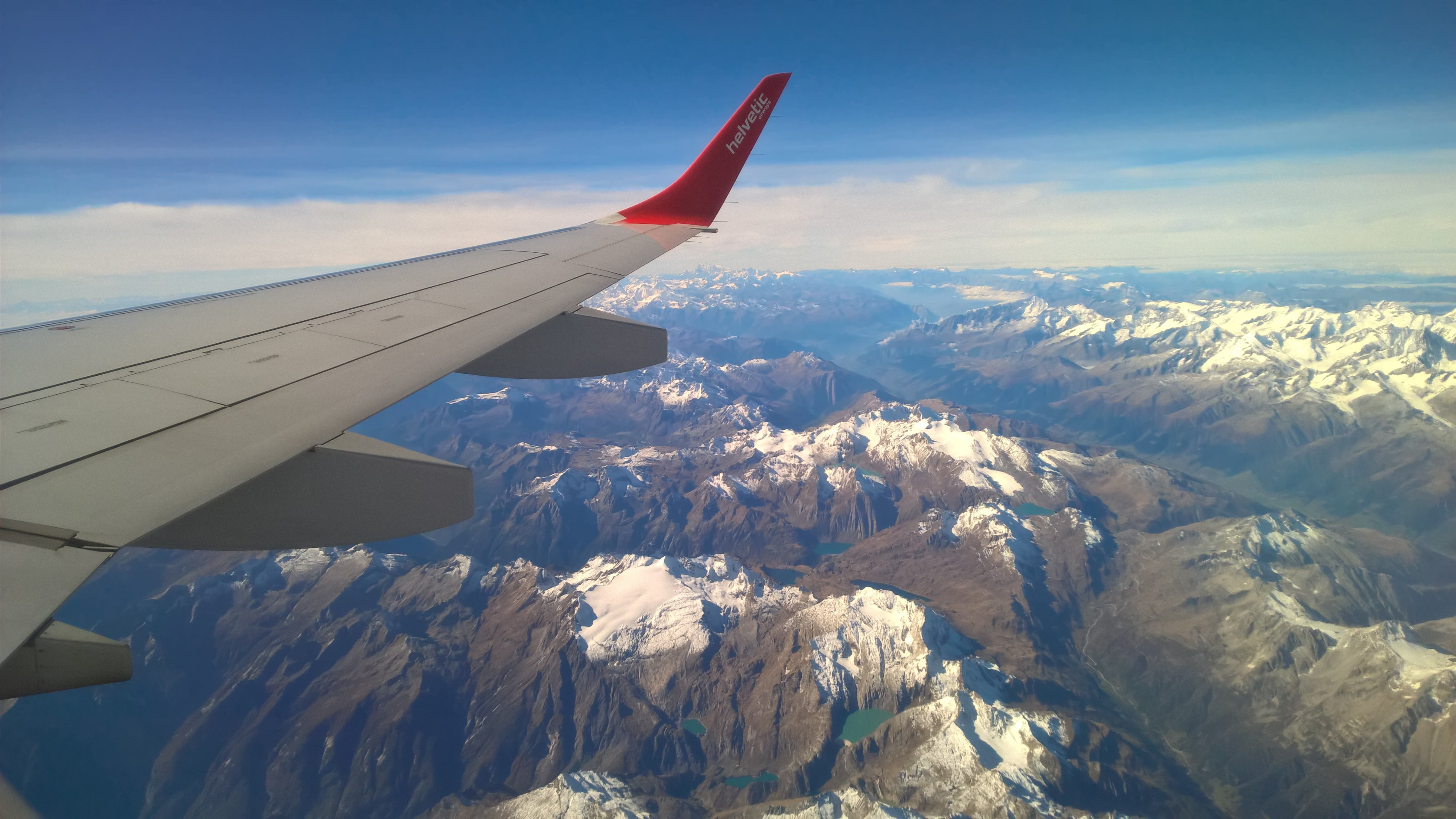
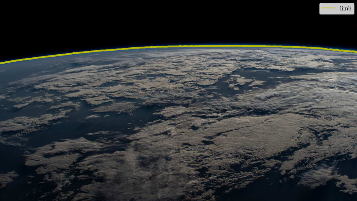
Example 1: Clear Horizon

Manual annotation goes quickly with clear horizons.

Example 2: Obstructions

User can avoid obstructions that can be tricky for automated methods.

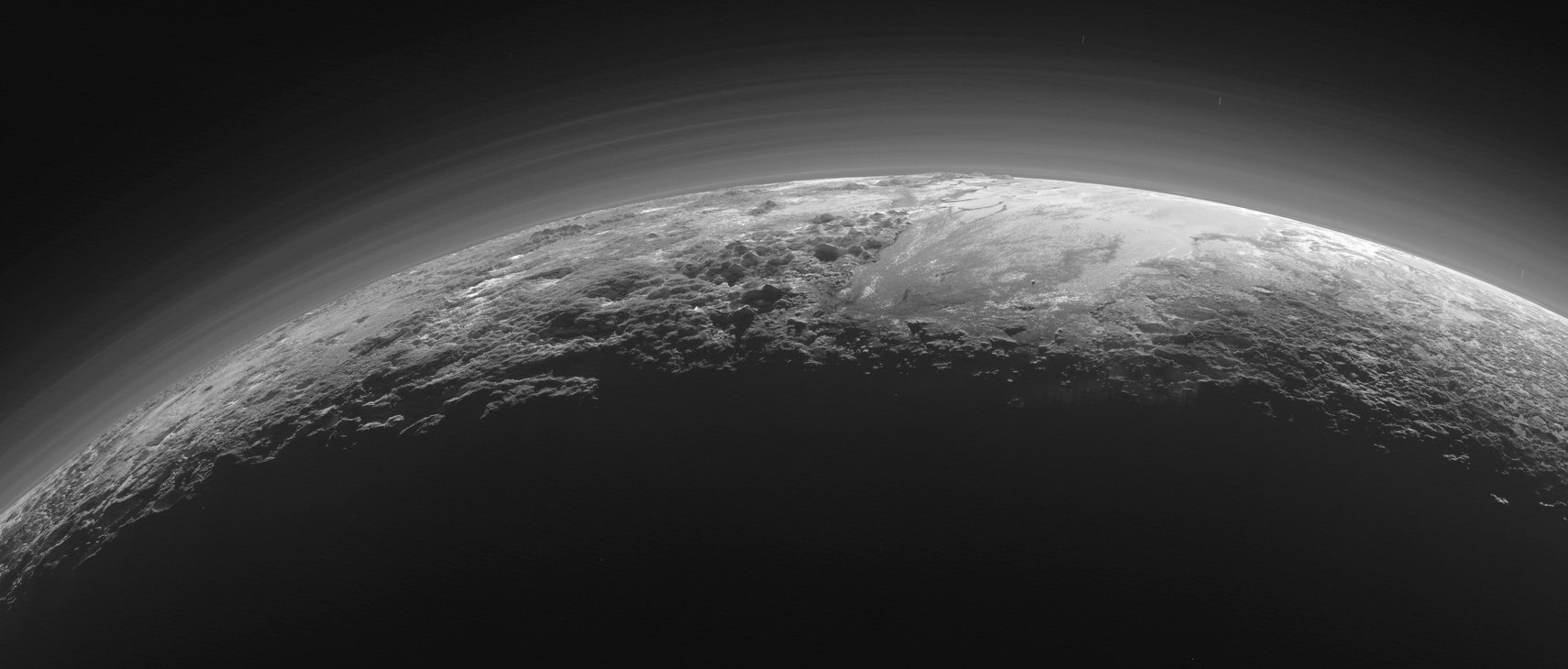
Example 3: Complex Scene

Anything besides a human would struggle with this.

Method 2: Gradient-Field Detection

Best for: Batch processing, clear horizons, reproducible workflows

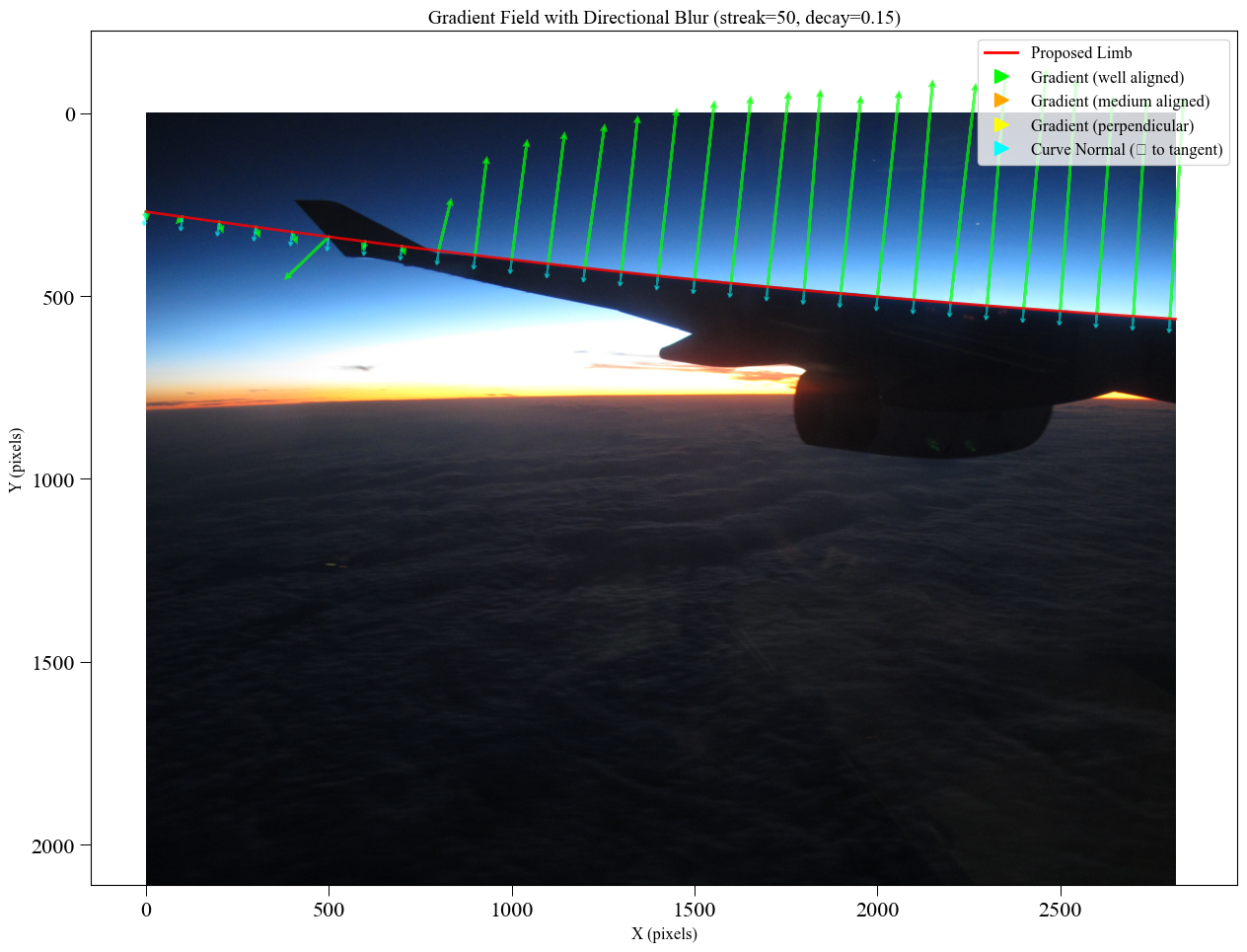
How It Works

Gradient-field detection skips explicit horizon detection entirely. Instead, it optimizes parameters directly on the image using brightness gradients perpendicular to the predicted horizon.

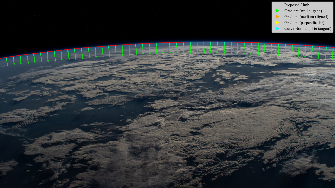
A ‘good’ horizon is one with high brightness gradient (flux) traversing its boundary.

The method uses multi-resolution optimization (coarse → fine) to avoid local minima.

Strengths:

✅ Fully automated - No user interaction require

✅ Lightweight - No ML models, low memory usage

✅ Reproducible - Same image → same result every time

✅ Fast - Processes images in around a minute

✅ Batch-friendly - Perfect for processing hundreds of images

✅ Multi-resolution - Robust to initialization

Limitations:

❌ Needs clear edges - Struggles with diffuse or gradual horizons

❌ Sensitive to obstruction - Horizon obsturctions can confuse it

❌ No visual feedback - You don’t see the detected horizon until after fitting

❌ Parameter tuning - May need to adjust smoothing parameters

When to Use

Use gradient-field when:

• You’re batch processing many images (10+)

• Horizons are sharp and well-defined

• You want reproducible results

• You don’t have time for manual annotation

• You want lightweight processing (no GPU needed)

• Images are clean with minimal obstruction

Example Usage

import planet_ruler as pr

# Load observation
obs = pr.LimbObservation("image.jpg", "config.yaml")

# Gradient-field optimization (no detection step!)
obs.fit_gradient(
    resolution_stages='auto',      # Multi-resolution: 0.25 → 0.5 → 1.0
    image_smoothing=2.0,           # Remove high-freq artifacts
    kernel_smoothing=8.0,          # Smooth gradient field
    minimizer='dual-annealing',
    minimizer_preset='balanced',
    max_iter=1000
)

# Note: No detect_limb() call needed!

Tip

Tuning parameters:

• Increase image_smoothing (2.0 → 4.0) for noisy images

• Increase kernel_smoothing (8.0 → 16.0) for hazy horizons

• Use prefer_direction="up" if above the horizon is darker than below

• More resolution stages (e.g., [8,4,2,1]) or minimizer_preset='robust' for difficult cases

Visual Examples

Inside the Process

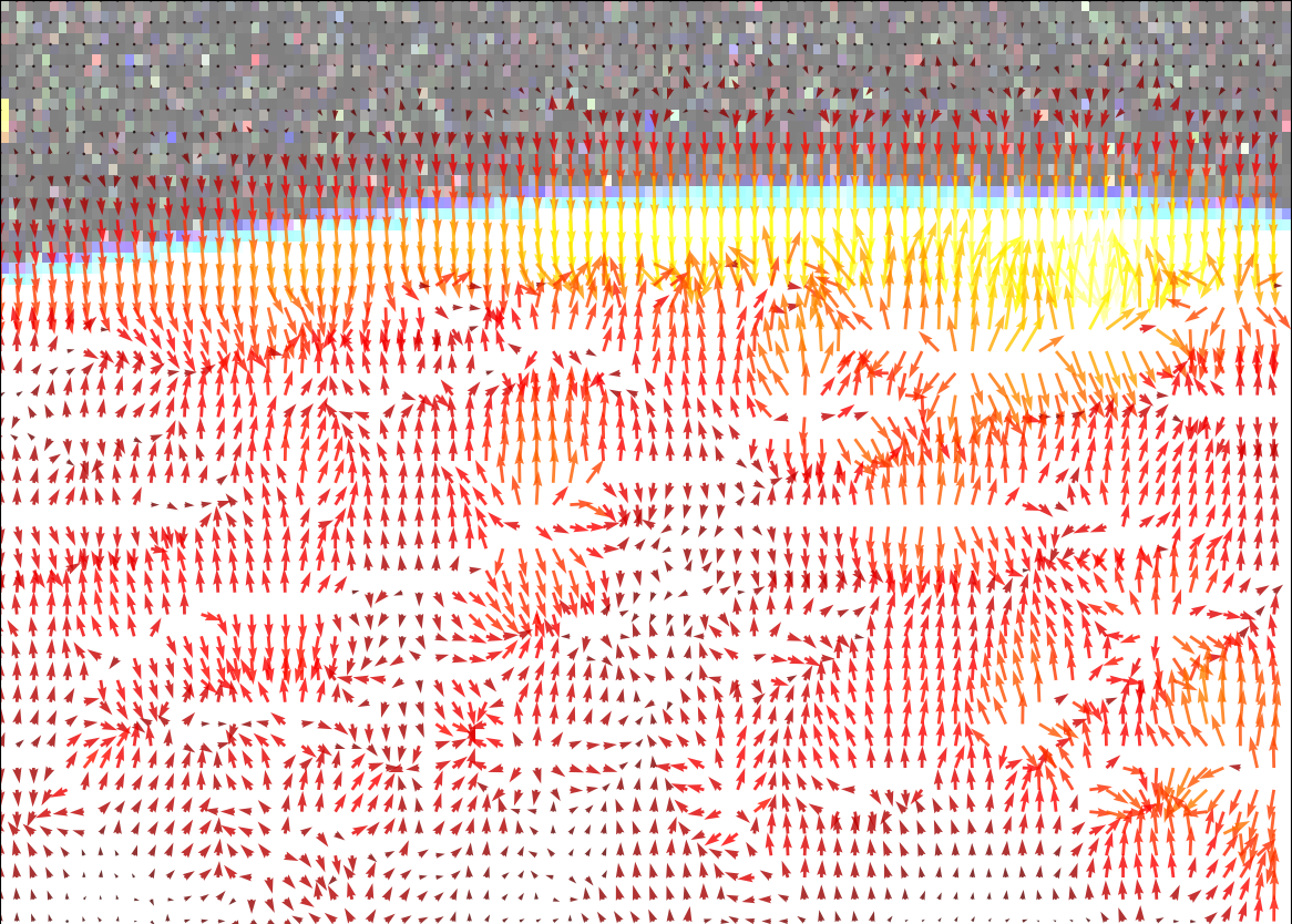
Raw image	Gradient field
Planet radius fitted	“Flux” through fitted radius

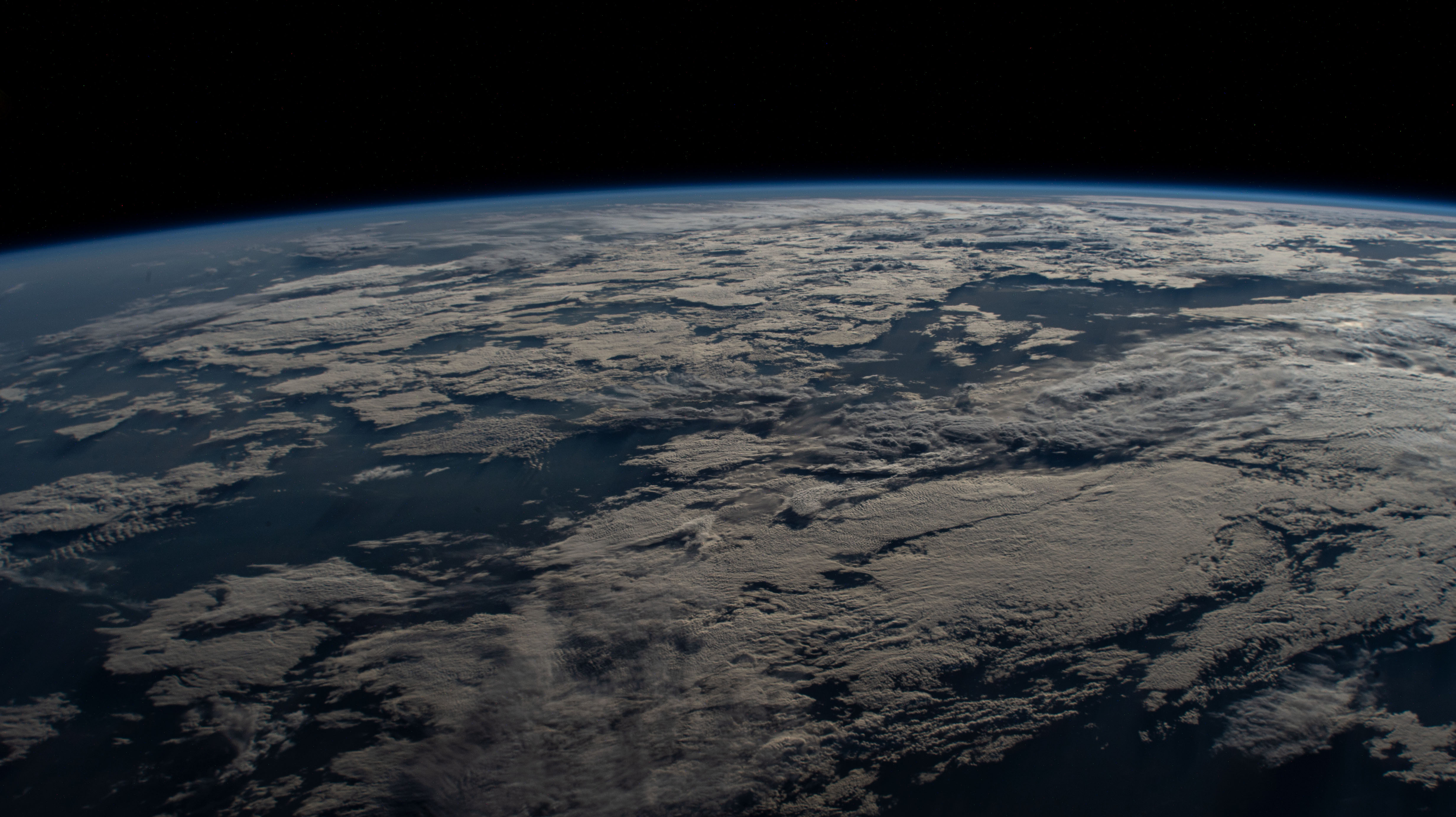
Example 1: ISS Earth Photo

Caption: Gradient-field works perfectly on clean spacecraft imagery.

Example 2: New Horizons Photo

Caption: Hazy atmospheric boundary detected accurately. Multi-resolution helps.

Example 3: Failure Case

In this case it may have been better to go with manual annotation…

Performance Notes

Typical timing (Intel i7, 2000x1500 image):

Resolution stages [4, 2, 1]:
- Stage 1 (500x375):     8 sec
- Stage 2 (1000x750):   12 sec
- Stage 3 (2000x1500):  20 sec
Total: ~40 seconds

Memory usage: <200 MB

Method 3: ML Segmentation

Best for: Complex scenes, when you have GPU + PyTorch installed

How It Works

ML segmentation such as Meta’s Segment Anything Model (SAM) can be used to automatically detect the planetary body. In automatic mode (interactive=False), the model assumes the two largest masks are the planet and sky and labels their boundary as the horizon.

Original

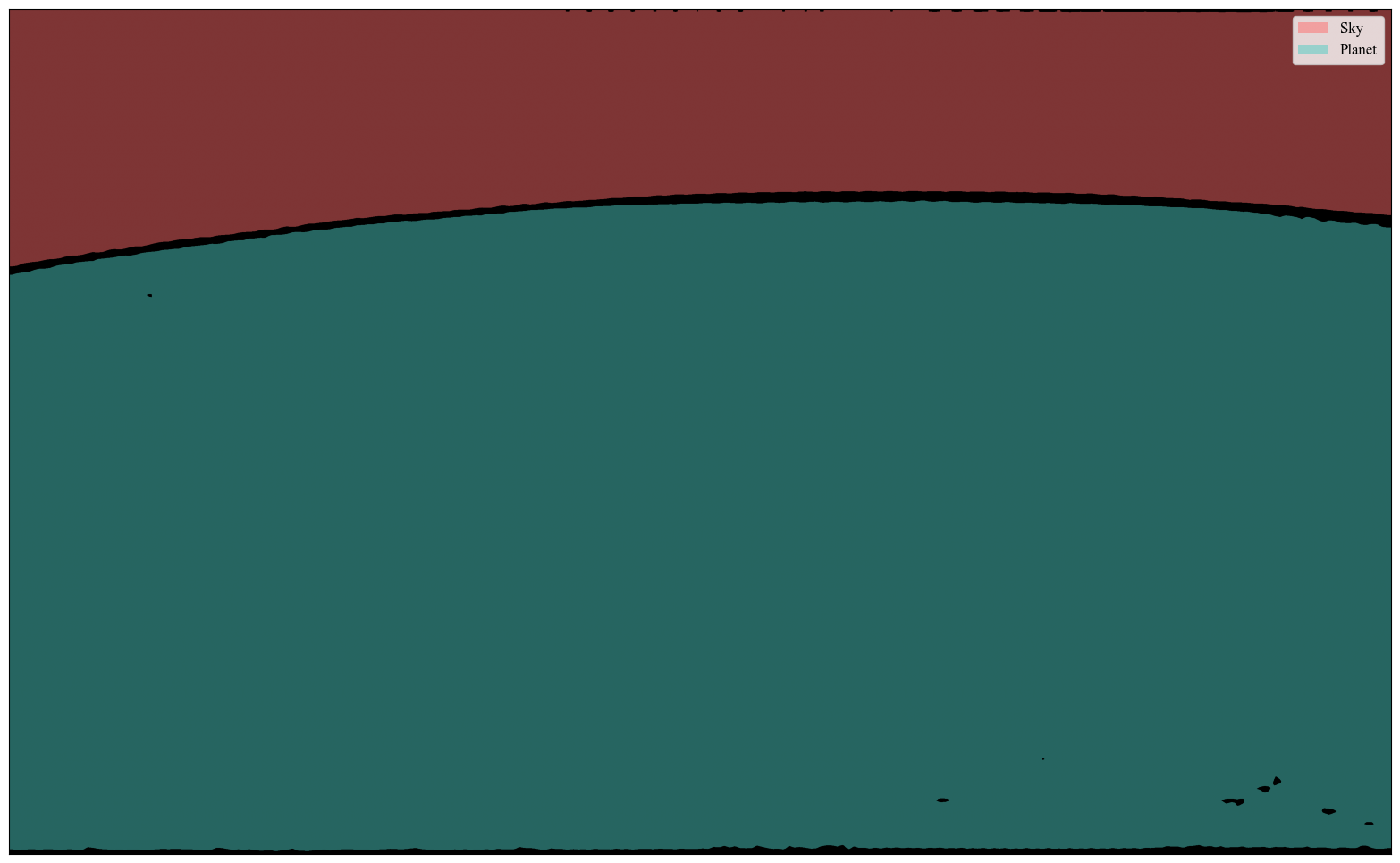
Segmented image

Detected limb

When set to interactive, however, the user is allowed to validate which masks belong to the sky and planet (or which to exclude) before the horizon is determined. This can help with obscuring objects like airplane wings or clouds. Note this method still isn’t foolproof – stay tuned for updates!

Original

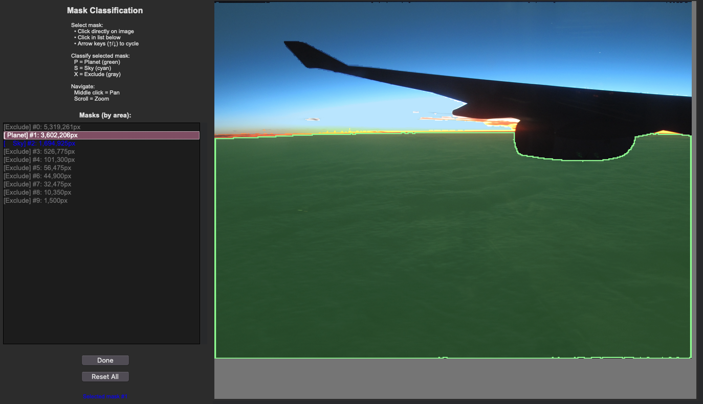
User Mask Annotation

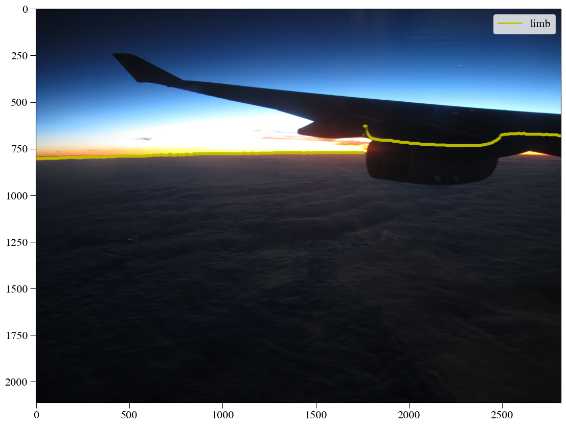
Detected limb

Strengths:

✅ Handles complexity - Can work with clouds, terrain, atmospheric layers

✅ Fully automated - Can run with zero user interaction

✅ Semantic understanding - “Knows” what a planet looks like

✅ Human-in-the-loop ready - Can leverage user annotations for increased accuracy

✅ Reproducible - Deterministic results

Limitations:

❌ Heavy dependencies - Requires PyTorch + SAM (~2GB model)

❌ Slow - 30-300 seconds per image (CPU) or 5-20 seconds (GPU)

❌ Memory hungry - Needs 2-4 GB RAM

❌ First-time setup - Model download takes 5-10 minutes

❌ Not always accurate - Can misidentify horizon with complex scenes

❌ Black box - Hard to understand why it makes certain decisions

When to Use

Use ML segmentation when:

• You have PyTorch and GPU available

• Scenes are complex (clouds, haze, terrain)

• You want to avoid manual clicking

• You’re willing to accept occasional failures

• Images have clear color/brightness differences at horizon

• You’re processing a moderate number of images (5-50)

Example Usage

import planet_ruler as pr

# First time only: model will auto-download (~2GB)
# This takes 5-10 minutes on first use

# Load observation
obs = pr.LimbObservation("image.jpg", "config.yaml")

# ML segmentation
obs.detect_limb(detection_method="segmentation")

# Always inspect the result!
obs.plot()

# If detection looks good, proceed
obs.fit_arc(max_iter=1000)

Warning

Always visually inspect ML segmentation results before fitting! The model can occasionally misidentify features as the horizon. If the detection looks wrong, use interactive mode or manual annotation instead.

Installation

# Install PyTorch (CPU version)
pip install torch torchvision --index-url https://download.pytorch.org/whl/cpu

# Install Segment Anything Model
pip install segment-anything

# For GPU support (faster, requires CUDA)
pip install torch torchvision --index-url https://download.pytorch.org/whl/cu118

Method 4: Sagitta (Arc-Height) Estimation

Best for: Quick radius estimates, warm-starting a subsequent arc fit

How It Works

The sagitta method estimates the planetary radius directly from the vertical “sag” of the horizon arc — the pixel distance between the highest and lowest points of the detected limb. It runs a fast 2-D optimizer over curvature and tilt and does not need differential evolution, making it much faster than a full arc fit.

Because it updates the parameter bounds automatically, it is especially useful as a first stage that narrows the search space for a subsequent fit_arc or fit_gradient call.

Strengths:

✅ Very fast — seconds rather than minutes

✅ No minimizer hyperparameters — works out of the box

✅ Warm-starts downstream stages — automatically tightens bounds

Limitations:

❌ Requires a detected limb — needs detect_limb() first

❌ Less precise than arc fit — use as a first stage, not final answer

When to Use

Use the sagitta method when:

• You want a fast sanity-check radius before committing to a full fit

• You want to warm-start a slower arc or gradient-field optimization

• You are processing many images and speed is critical

Example Usage

import planet_ruler as pr

obs = pr.LimbObservation("image.jpg", "config.yaml")
obs.detect_limb(detection_method="manual")

# Stand-alone sagitta estimate (fast)
obs.fit_sagitta()
print(f"Quick radius estimate: {obs.best_parameters['r']/1000:.0f} km")

# Or chain sagitta → arc for speed + accuracy (recommended combo)
obs.fit_limb(stages=[
    {"method": "sagitta"},
    {"method": "arc", "minimizer": "differential-evolution",
     "minimizer_preset": "balanced"},
])
print(f"Final radius: {obs.best_parameters['r']/1000:.0f} km")

Tip

The sagitta → arc chain is the recommended default workflow for manual annotation in 2.0. Sagitta quickly finds a good starting radius and tightens the parameter bounds; the arc fitter then refines it precisely.

Combining Methods

Best Practices Workflow

For critical measurements, use multiple methods and compare:

import planet_ruler as pr
from planet_ruler.uncertainty import calculate_parameter_uncertainty

results = {}

# Manual annotation → arc fit
print("\nTrying manual method...")
obs = pr.LimbObservation("image.jpg", "config.yaml")
obs.detect_limb(detection_method='manual')
obs.fit_arc()
results['manual'] = obs

# Gradient-field: no detection step needed
print("\nTrying gradient method...")
obs = pr.LimbObservation("image.jpg", "config.yaml")
obs.fit_gradient(resolution_stages='auto')
results['gradient'] = obs

# ML segmentation → arc fit
print("\nTrying ML segmentation method...")
obs = pr.LimbObservation("image.jpg", "config.yaml")
obs.detect_limb(detection_method='segmentation')
obs.fit_arc()
results['ml'] = obs

# Compare results
print("\nMethod comparison:")
radii = {}
for name, obs in results.items():
    radius_result = calculate_parameter_uncertainty(
        obs, "r", scale_factor=1000, method='auto'
    )
    radii[name] = radius_result['value']
    print(f"  {name}: {radius_result['value']:.1f} km")

# Check consistency
import numpy as np
values = list(radii.values())
print(f"\nSpread: {np.max(values) - np.min(values):.1f} km")
print(f"Mean: {np.mean(values):.1f} km")
print(f"Std: {np.std(values):.1f} km")

Troubleshooting Decision Guide

If Your Results Look Wrong

Problem: Manual annotation gives inconsistent results

• Solution: Click points with more care

• Solution: Use zoom/stretch features for precision

• Solution: Try gradient-field for comparison

Problem: Gradient-field result is way off

• Check: Is horizon clearly visible and sharp?

• Check: Are there clouds or haze at horizon level?

• Solution: Increase smoothing parameters (image_smoothing=4.0)

• Solution: Add more resolution stages [8,4,2,1]

• Fallback: Use manual annotation

Problem: ML segmentation detects wrong features

• Check: Visually inspect with obs.plot() before fitting

• Solution: Try interactive mode to refine masks

• Solution: Increase smoothing after detection

• Fallback: Use manual annotation (always reliable)

Summary

Choose Manual Annotation if:

• You want maximum accuracy

• You’re analyzing 1-10 images

• You’re teaching or learning

• Image quality is poor

• You can spare 1-2 minutes per image

Choose Gradient-Field if:

• You’re batch processing many images

• Horizons are clean and sharp

• You want reproducible results

• You don’t have GPU/PyTorch

• Speed is important

Choose ML Segmentation if:

• You have PyTorch + GPU installed

• Scenes are complex but horizon is visible

• You want to experiment with AI methods

• You’re willing to visually inspect results

• You have time for model download (first time)

Use Sagitta as Stage 1 when:

• You want a fast warm-start before a slower arc fit

• You need a quick sanity-check radius estimate

• You are batch processing and want to reduce full-fit time

When in doubt: Start with manual annotation followed by a sagitta → arc staged fit (obs.fit_limb(stages=[{"method": "sagitta"}, {"method": "arc"}])). This is the recommended default workflow in 2.0.

Next Steps

• Try Prerequisites for a complete walkthrough with manual annotation

• See When to Use Gradient-Field for gradient-field examples

• Check Examples for real-world comparisons

• Read API Reference for advanced configuration options